Analyzing Ordinal Data in SAS using the Binary, Binomial, and Beta Distribution.

Author(s): Dr. Marc Jacobs

Originally published on Towards AI the World’s Leading AI and Technology News and Media Company. If you are building an AI-related product or service, we invite you to consider becoming an AI sponsor. At Towards AI, we help scale AI and technology startups. Let us help you unleash your technology to the masses.

This will post will build on previous posts — an introductory post on PROC GLIMMIX and a post showing how to analyze ordinal data using the ordinal and multinomial distribution. This post will extend those posts by analyzing the same dataset — diarrhea scores measured in pigs across time. Here, diarrhea is measured subjectively using an ordinal scoring system.

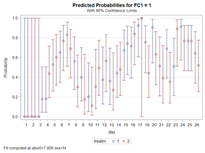
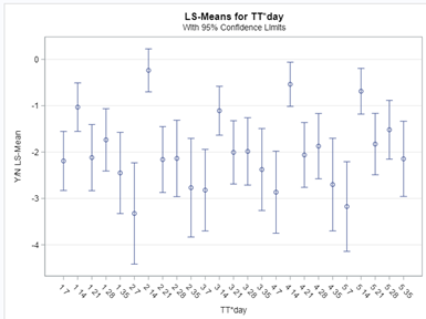
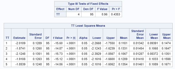
So, let's move to the Binomial distribution and its continuous counterpart, the Beta distribution. The Binary & Binomial distributions both deal with discrete proportions and transform them into probabilities/proportions. Below you can see an example coming from an ordinal model using the cumulative probability distribution of the cumlogit link.

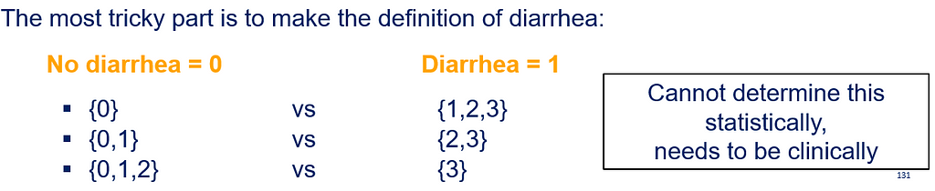
However, sometimes it is just not possible to estimate the effect of a treatment in an ordinal manner. Here, scores 2 and 3 add less than 15% to the total scale. Hence, it would perhaps be wise to combine them and to compare scores — for instance by aggregating four groups into two (0 & 1 vs 2 & 3). If you do so, you need to also specify what diarrhea is exactly because you can do 0 &1 vs 2 & 3. Or, you can do 0 vs 1 & 2 & 3. Statistics won't help you here to make that decision, it has to come from content knowledge.

Now, if you want to analyze a binary division you need to determine if you want to analyze it as a proportion or as a rate:

1. Proportion = ratio of the same two metrics → diarrhea / total feces
2. Rate = ratio of two distinct metrics → diarrhea/total days measured

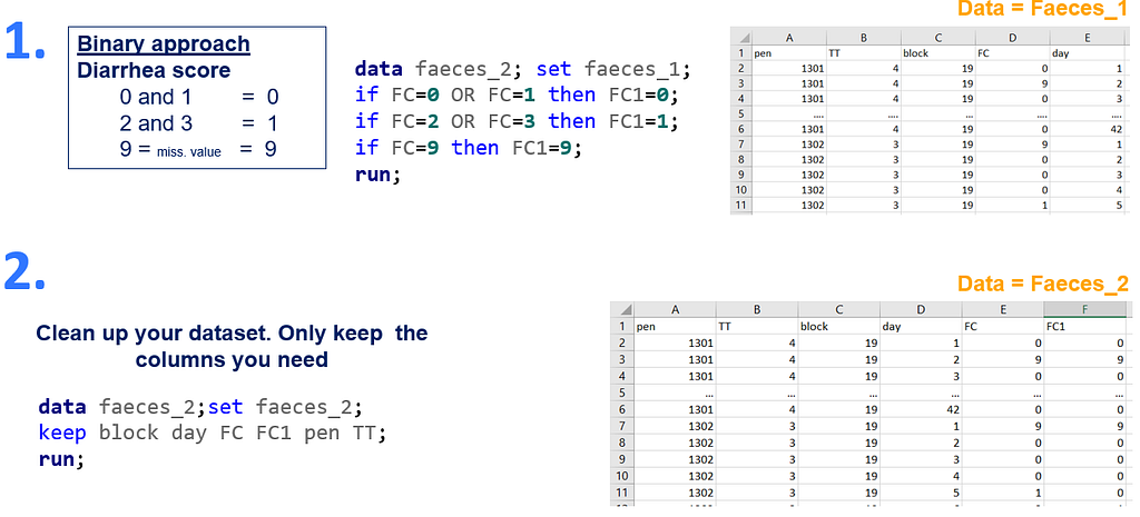
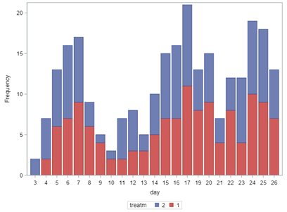
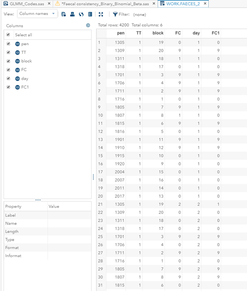
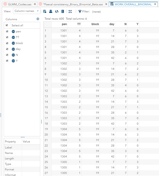
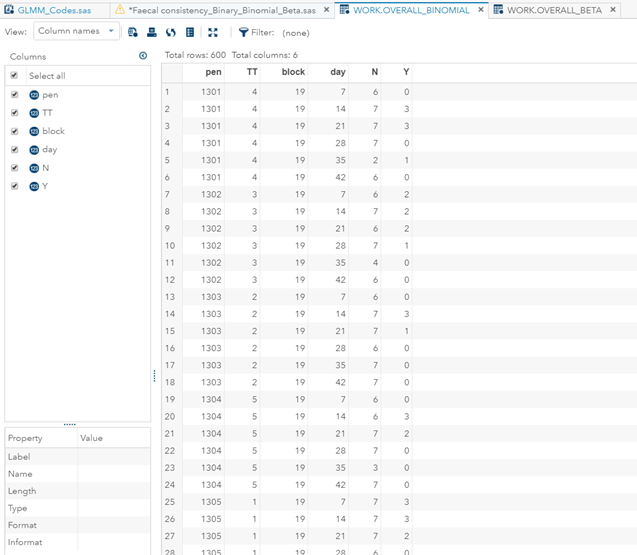
In terms of data management, the data needs to be made appropriate for analysis by a binary or binomial distribution. Since Binary / Binomial can deal with the time component (unlike the Ordinal or Multinomial distribution), we want to create a dataset that can accommodate this kind of analysis. Below you see the final dataset in which we have, per pen, the treatment, block, day, and feacal score. There is no longer a frequency metric included.

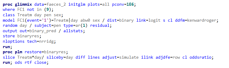
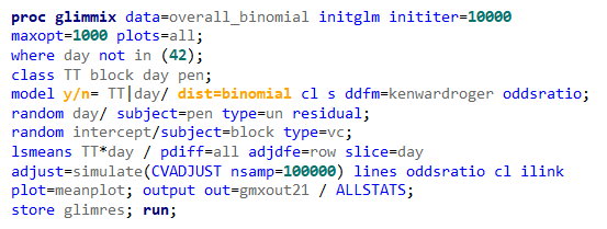
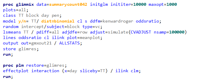
Now, let's move on to the actual modeling. As I said, I will use the binary distribution and the logit link. That is the same link as I used for the Ordinal / Multinomial Model. It also means that comparisons will be done using the Odds Ratio.

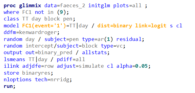
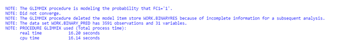
The code for the Binary distribution did not run which is not strange, since it often does not run. This is because of the way the model needs to assess the variance in the data — by looking between rows. If there is not enough variance, or if there is not enough data, the model just won’t converge. No matter what.

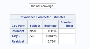
So, let's try the Binary distribution on a different dataset. Most of the time, there is just not much you can do from a model perspective if the data does not hold the granularity needed.

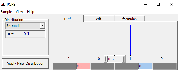
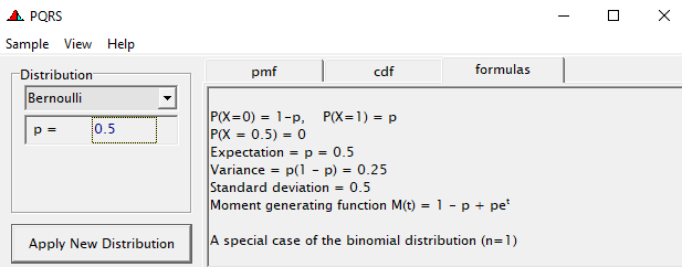
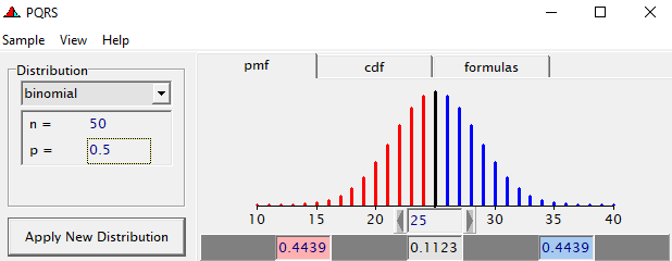
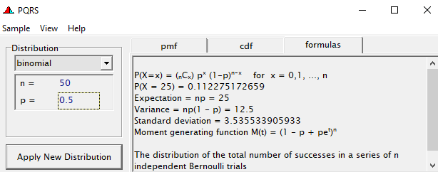
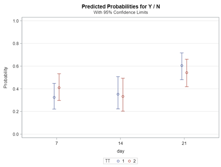
Now, let's venture from the Binary distribution to the Binomial distribution. They are very much the same, except that in a Binary the N=1 whereas for the Binomial the N=N — you conduct multiple independent trials from which to assess probability. The Binary distribution is often referred to as the Bernoulli distribution.

To go from using the Binary (or Bernoulli distribution) to using the Binomial distribution, we need to change the dataset to accommodate the Y/N necessity — the number of wins given the number of games. Of course, the Y/N is already a proportion and thus a probability distribution by itself.

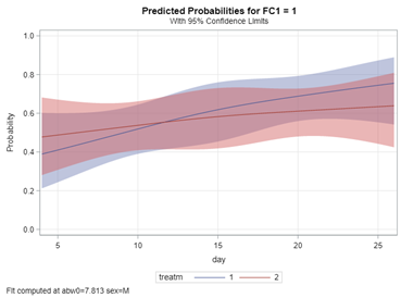
Below you can see the transformation from the dataset used for the Binary distribution to the dataset used for the Binomial distribution. I am still trying to model across time, but this time I had to aggregate the data at the week level. This will make the model more stable.

In conclusion, there is not enough variation within this dataset to get a proper model and I detected a lot of boundary values. In addition, the animals were challenged with sub-optimal feed which means that the challenge was not strong enough to get valuable diarrhea results. In other words, the dataset does not contain the level of granularity that I need.

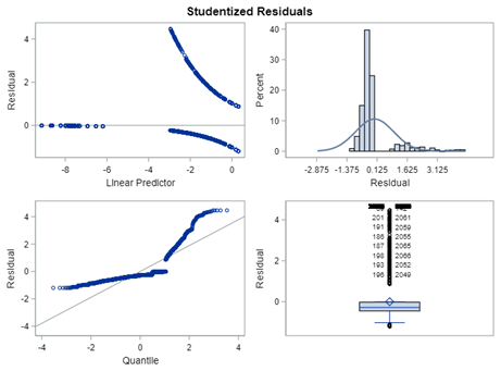
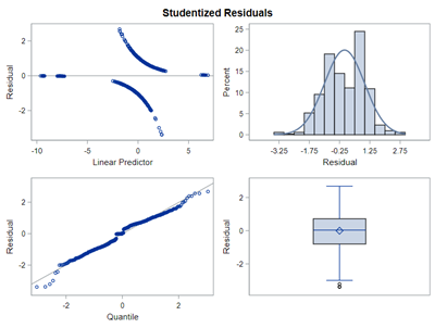
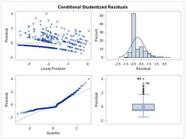
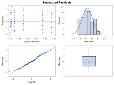
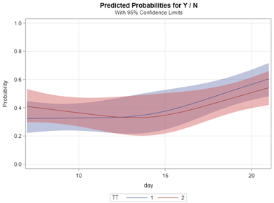
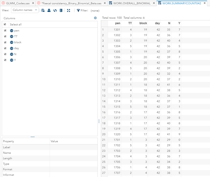
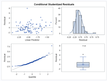
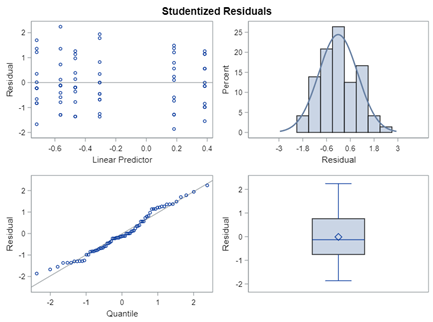
So let's go and try on a different dataset with the same type of modeling. Below you can see the results. Once again, don’t focus too much on the residuals. Even if they look very ‘ Normal’ now, you should not expect them to be. We are not modeling data using a Normal Distribution.

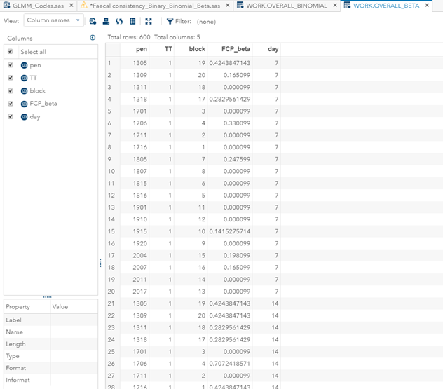
Now, how would it look like if I would not model per week the old dataset, but just model it overall — the proportion of diarrhea within 42 weeks? To do so, I need to transform the data until I end up with the one on the right.

So, analyzing diarrhea scores via a binary/binomial distribution warrants the decision to specify which scores constitute diarrhea and which do not — it has to be binary. Binary data is yes / no data in its rawest form and is most difficult to analyze. Binomial data is data in the form of a numerator/denominator and often gives you are more stable model. Analyzing the data in a binary/binomial way warrants the transformation of a dataset.

Let's see how far we can go using its continuous counterpart — the Beta distribution.

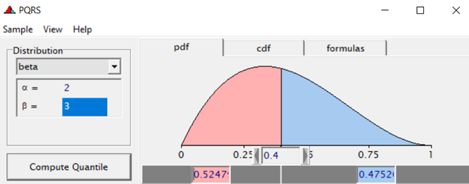
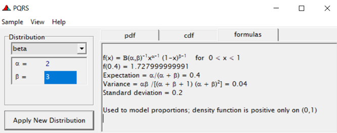
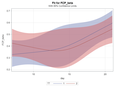
Modeling diarrhea using the Beta distribution means that you are venturing into the world of continuous proportion. Below, you can see an example of the Beta distribution and its two parameters — alpha and beta. As you can immediately see, the alpha and beta can be inserted separately, but they are still entwined. This becomes clear when you look at the formulas for the mean and the variance.

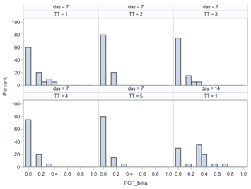
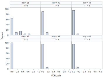
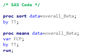
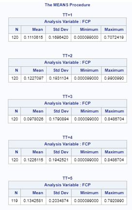
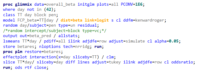
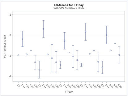
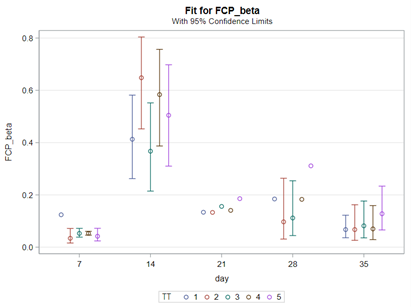
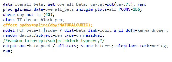
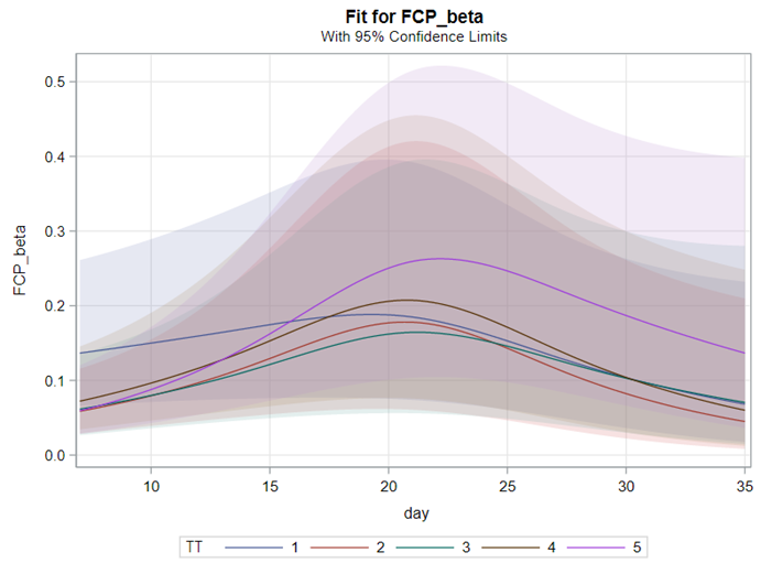
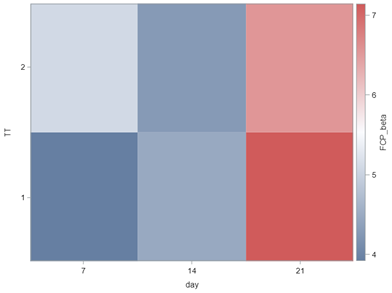
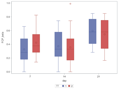
Lets again use a different dataset to see if we have more success in using the Beta this time.

In summary, the Beta Distribution models proportions, just like the binary and the binomial distribution. Compared to the binary/binomial distribution, the beta distribution models proportions on a continuous spectrum. To use the beta distribution, you need to have proportions in the dataset, and no proportion can be 0 or 1. Compared to the other distributions, the beta distribution is the easiest to model and the easiest to understand.

Hope you enjoyed it!

---

Analyzing Ordinal Data in SAS using the Binary, Binomial, and Beta Distribution. was originally published in Towards AI on Medium, where people are continuing the conversation by highlighting and responding to this story.

Join thousands of data leaders on the AI newsletter. It’s free, we don’t spam, and we never share your email address. Keep up to date with the latest work in AI. From research to projects and ideas. If you are building an AI startup, an AI-related product, or a service, we invite you to consider becoming a sponsor.

Published via Towards AI