Analyzing Ordinal Data in SAS using the Multinomial Distribution.

Author(s): Dr. Marc Jacobs

Originally published on Towards AI the World’s Leading AI and Technology News and Media Company. If you are building an AI-related product or service, we invite you to consider becoming an AI sponsor. At Towards AI, we help scale AI and technology startups. Let us help you unleash your technology to the masses.

This post is an extension of an earlier introductory post I made on using Generalized Linear Mixed Models in SAS.

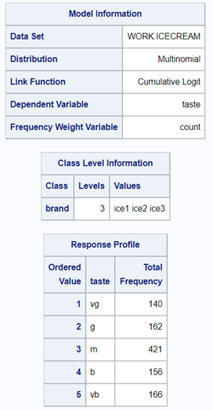
Below, I will use a dataset containing the diarrhea scores of pigs to show how to analyze ordinal data. Before doing so, one has to consider that the assessment of diarrhea scores is done in a subjective way, using raters, who rate diarrhea on a score from 0 to 3 in steps of 1 — 0,1,2,3. A nine equals the absence of feces from which to assess diarrhea. It is not immediately clear if that actually means that there is no diarrhea or just plain absence. It can also have an effect on the analysis itself.

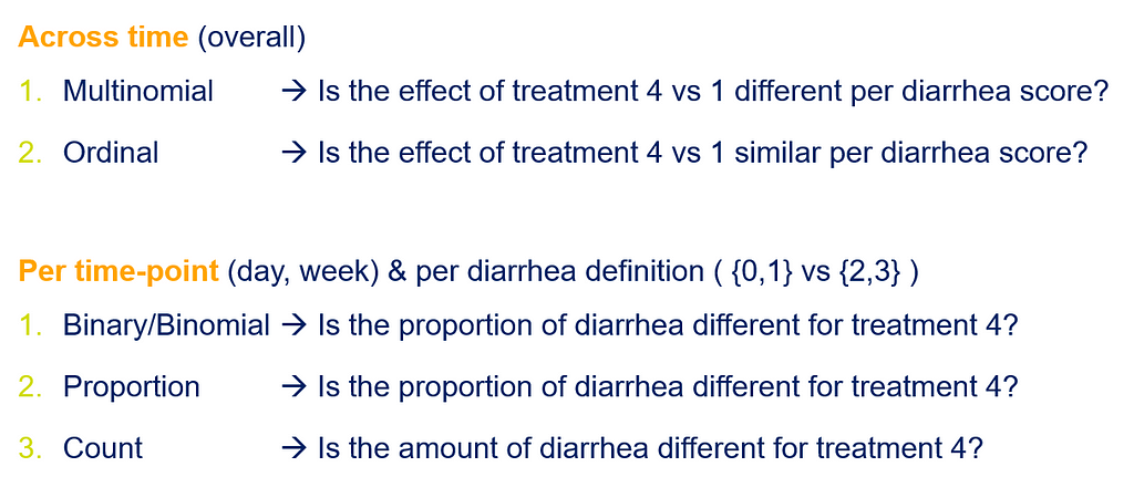
Ordinal data can be analyzed in multiple ways, of which we show the ordinal and multinomial way in this post. The type of analysis you will use depends on your assumptions, the specific question you would like to answer, and what the model is able to accommodate.

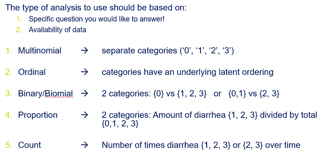
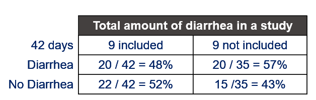
Diarrhea is a discrete outcome and as such should be treated as a proportion and not a continuous distribution with a true mean. Renaming the levels of diarrhea from {0, 1, 2, 3, 9} into {A, B, C, D, Z} would solve the confusion. Diarrhea can be measured in multiple ways the choice of which should depend on the:

1. the specific question you want to be answered
2. availability of data

Let's do some actual analysis and use a dataset that looks like this, to start with.

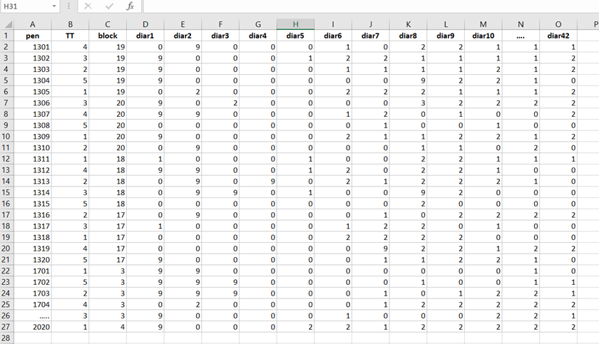
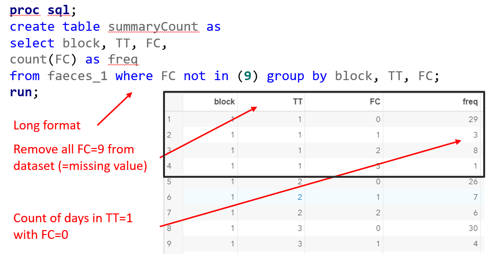
The multinomial approach is perhaps the easiest, to begin with. Remember, Ordinal and multinomial models cannot handle repeated data. Thus only total periods may be used (f.e. 0–42, 0–14, etc.). So, to use ordinal/multinomial models, specific data management is required:

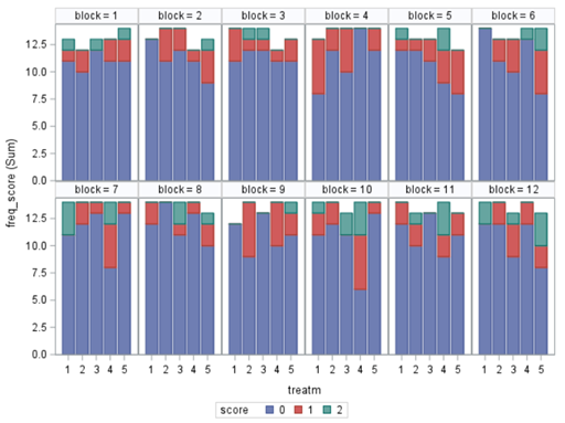
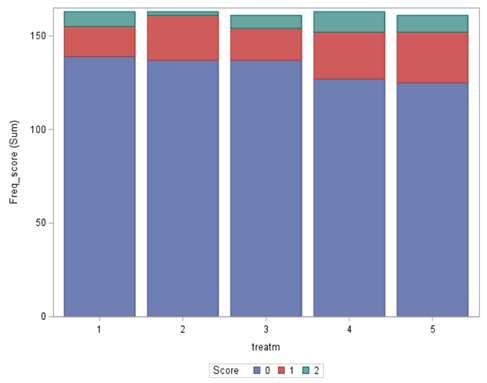
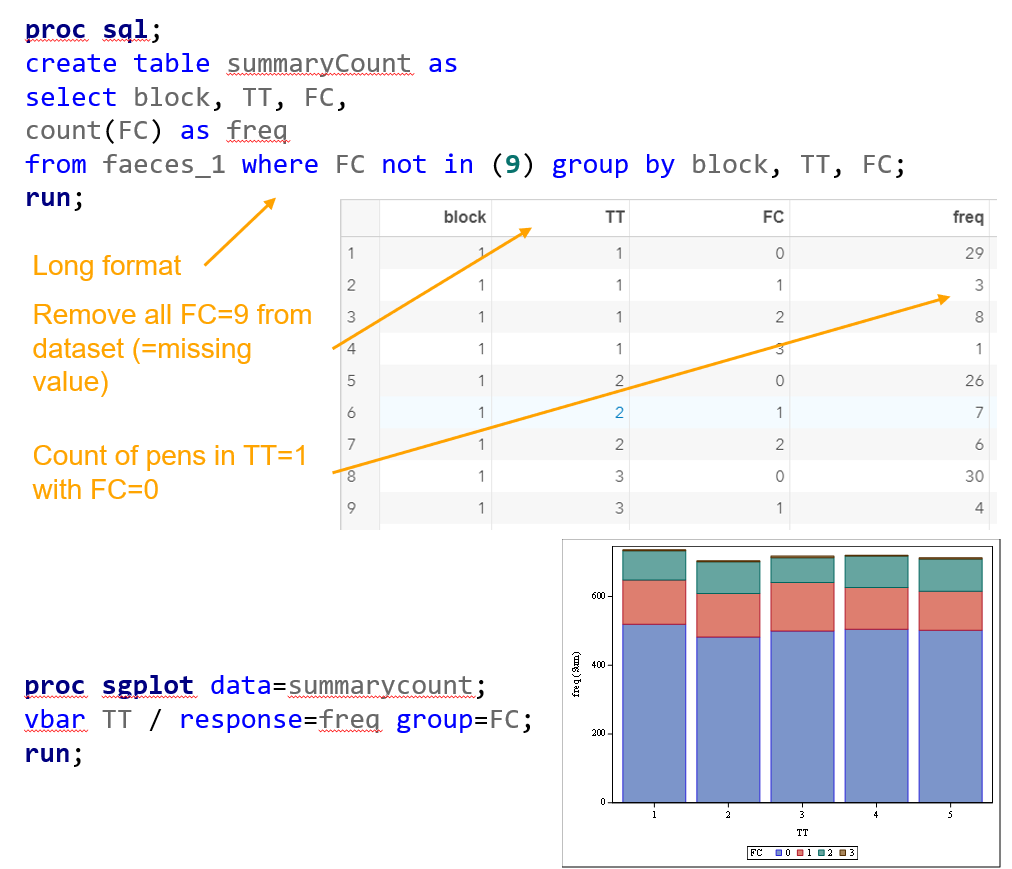
1. per Block, Treatment & Fecal Consistency Score, the frequency needs to be calculated and put in the model.
2. In case of fecal consistency, category ‘9’ (FC=9) is removed, as these are often deemed missing values (see earlier discussion points)

Below you see the PROC SQL command to transform the data in a dataset that is necessary for both multinomial and ordinal modeling. The trick is to get frequencies per category per treatment per block.

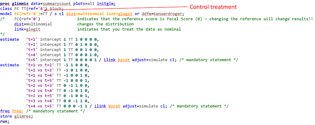
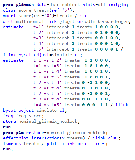
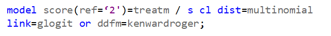
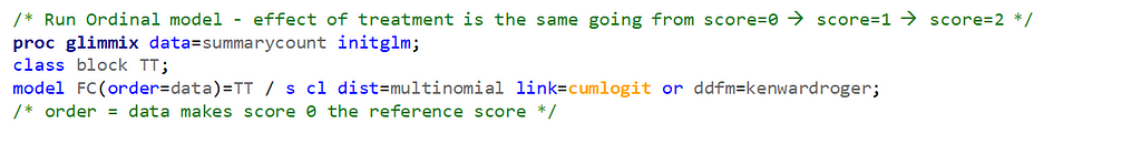
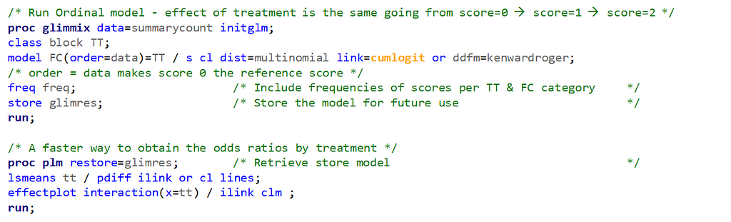
Below, you see the full code used the model the multinomial. The distribution is set at multinomial, but this is also the case if you want to model using the ordinal approach. Hence, the key is the link function, set here at glogit and will be set to clogit for the ordinal approach — glogit stands for generalized logit and means that we will estimate the proportions separately. Treatment four is set as the reference treatment. For the estimates, you need to use the bycat function to get estimates per category of the feacal consistency score.

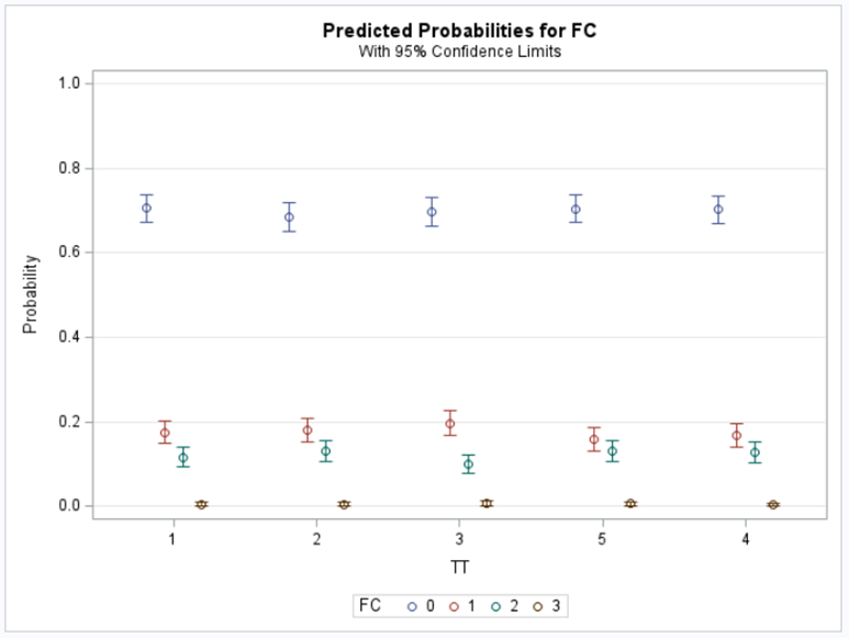
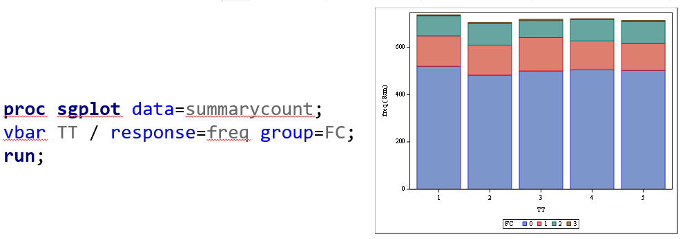
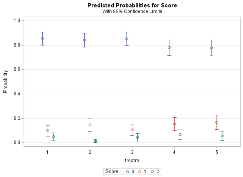
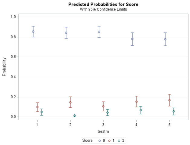
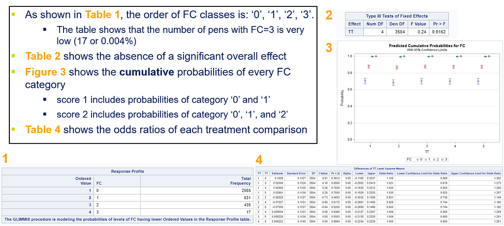
Plotting the results is often a better way of getting to terms with your model. This graph shows the probabilities for each of the diarrhea scores across treatments. From the graph you can see that:

1. Score 3 is almost absent
2. Score 0 is most present
3. Treatment difference seems to be most present in score 2

To understand the Odds Ratios from the previous table, you need to get comfortable with proportions. So, let's use another example but to do so, we need to once again transform the data to let PROC GLIMMIX process it.

And below the same code, we saw before.

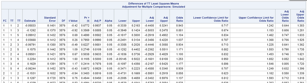
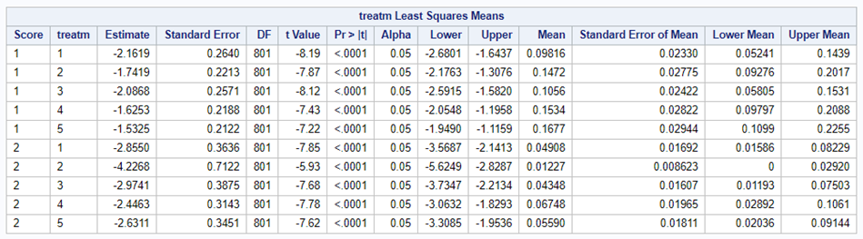
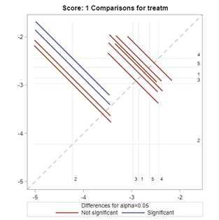
Now, the plot above is quite easy to interpret but of course, you need to have actual numerical estimates to make sense of the effect size of the differences between treatments. In a multinomial model, the interpretation depends on the choices you made — even more than for any other kind of model.

So, as you can see, the table is a bit different than normal, but we already knew that. Comparisons are made per score category. But, if you look more closely, you can see that score 0 is missing. That is because it is the reference score. If you want to have specific estimates for score=0, then you need to set a different reference score.

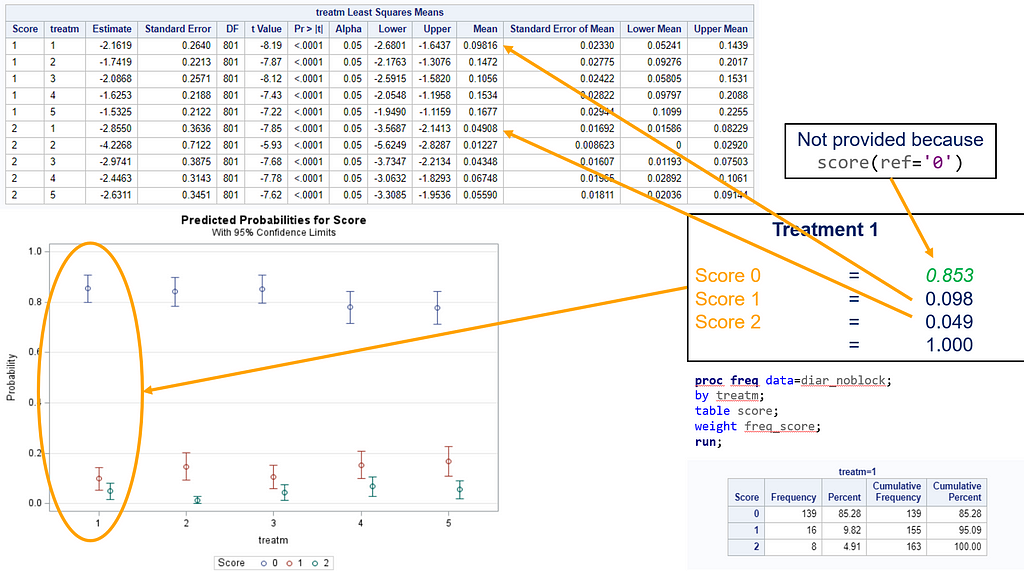
For the rest, it is pretty much straightforward. You get an estimate and a mean per an estimate, of which the mean is the probability. Once we go towards direct comparisons and treatment differences, you will have to deal with Odds Ratios again.

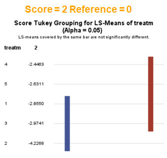
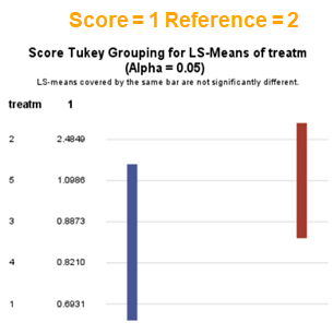
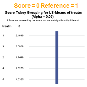
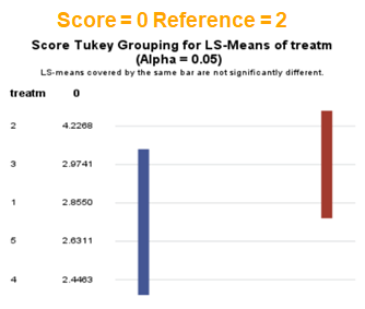
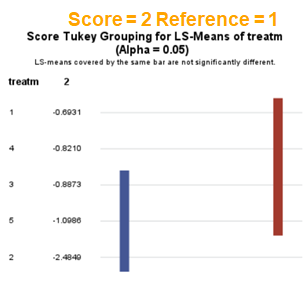
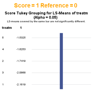
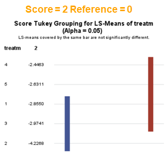
The influence of the reference score is easiest done by repeating the analysis, but by changing the reference score. Below, you see the probability plots for reference score zero en two. Now, please look closely and see that the actual probability plot does NOT change. That is because it cannot change. However, the estimates do differ, because the scores are compared to a DIFFERENT reference score.

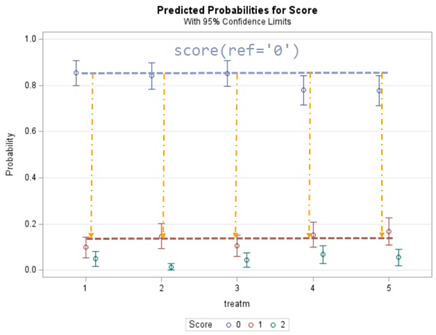
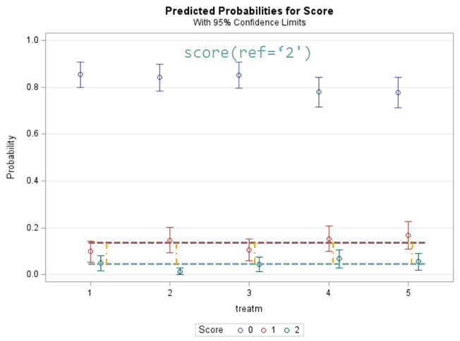
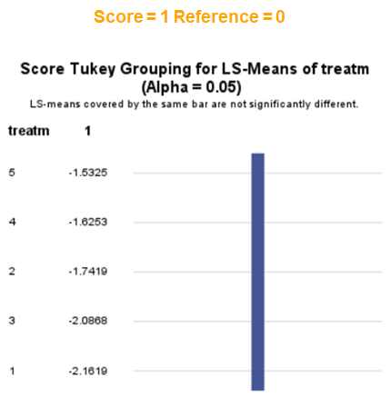
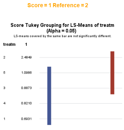
Below you can see what changing the reference score does for interpretation. It is quite something, so be careful if you look at these plots. In fact, I would like to advise you to only look at these plots in conjunction with the overall probability plot.

In summary, when analyzing diarrhea scores, the multinomial model is the most straightforward as it looks into the scores if they are mutually exclusive, and analyzes the treatment effect per score category. Beware, the reference score affects the results so keep thinking in terms of probabilities — graphs help — and in terms of odds ratios which are not intuitive. You could run the model multiple times, changing the reference score and treatment to get the full picture. Another caveat is that you cannot analyze the data in a repeated measures way — only suitable for the total period.

Now, let's move to the ordinal approach.

The ordinal model is built on the same foundation as the multinomial model, however, it does approach the data quite differently. In fact, the ordinal model builds in assumptions to make analyses and comparisons more easy and direct. Let's see if that truly is the case.

The majority of multi-level variables are ordinal which means that categories have a specific ordering although the “distance” between the levels is not clear. However, the categories are man-made and there is no actual underlying theoretical distribution. When using an ordinal model, you however do assume that there is a latent continuous variable underneath its categories. You also assume the Proportional Odds Assumption which is often not met. One way to defend the use of an ordered model is to say that underneath the observed scores there is a latent variable, Y*. This latent variable has thresholds, and crossing a threshold will place you in a different category. This is why an ordinal model is often called a ‘threshold model’. As a result, an ordinal model will come up with a single equation for Y*. This is also directly the difference with the multinomial model which allows for more than one equation since it treats the categories as separate

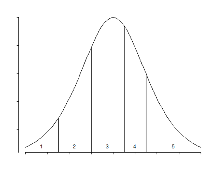
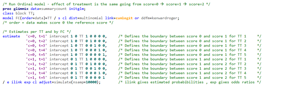
In an ordinal model, the only parameter that changes is the intercept. The fixed effects remain the same for each category. The intercept defines the boundaries between categories when the linear predictor is zero. Changes in the linear predictor move the boundaries together so that the distance between them remains CONSTANT!! This is the definition of the Proportional Odds assumption

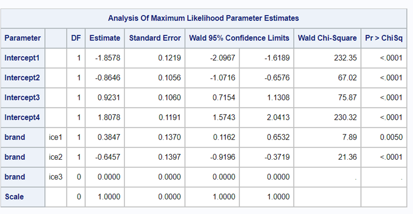
It is the intercept that determines the threshold for the next category. Hence, in a five-category outcome variable, we have four intercepts as you can see in the example below.

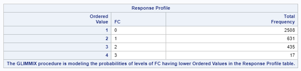
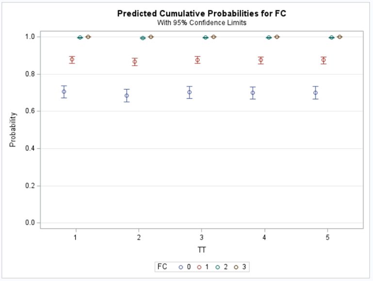
The best way to deal with complex math is to look at this plot — the cumulative probability plot. It shows the cumulative distribution of the frequencies. Here, it is clearly visible that score 0 is most frequent and that scores 2 and 3 add only a little. Hence, it is perhaps best to combine scores 1, 2 & 3 vs score 0

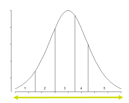
The key assumption to the proportional odds model is that the relationship BETWEEN categories remains the SAME. Hence, probabilities are not category-specific and treatment effects move the boundaries between categories as a group. As such, the odds ratios of a treatment effect for NOT SEVERE vs SEVERE are the same as for SEVERE vs VERY SEVERE.

Remember, an ordinal model tries to find a linear predictor that will predict the change from one category to the next, but the probabilities are not category-specific. We need to test this assumption using PROC GLIMMIX

If the assumptions of the ordered cumlogit model are met, then all of the corresponding coefficients (except the intercepts) should be the same. The assumptions of the model are therefore sometimes referred to as the parallel lines or parallel regressions assumptions

In summary, assuming that the data is ordinal means that there is a certain ordering of the discrete data. The specific ordering is determined by a latent continuous distribution. The data for the ordinal approach needs the same setup as for the nominal approach. Results show the effect of the treatment, regardless of the specific score. Hence, there is no reference to take into account. Checking if the proportional odds assumption was upheld is tricky.

I hope you liked this post! More to come!

---

Analyzing Ordinal Data in SAS using the Multinomial Distribution. was originally published in Towards AI on Medium, where people are continuing the conversation by highlighting and responding to this story.

Join thousands of data leaders on the AI newsletter. It’s free, we don’t spam, and we never share your email address. Keep up to date with the latest work in AI. From research to projects and ideas. If you are building an AI startup, an AI-related product, or a service, we invite you to consider becoming a sponsor.

Published via Towards AI