Image Processing using Morphological Operations

Last Updated on February 3, 2021 by Editorial Team

Author(s): Ralph Caubalejo

Computer Vision, Programming

Morphing Time!

One of the most essential image processing techniques out there is the so-called morphological operation.

As the name suggests, we use morphological operation in cleaning and correcting out the images. Normally, morphological operations are done after convolving an image to a specific kernel or spatial filter. Since the result of the spatial filtering is an image that shows different attenuated features, we would want them to be correct as a whole.

Sometimes, the resulting filtered image has broken lines or maybe joining other features that should be joined. This is where we use morphing. We again use a sort of structuring element and match it to the filtered image so that it can relate a pixel to its neighbor pixels. The result of the morphological operations are images that are more precise and more correct for application on the specific problem.

To better understand the concept, let us go fast on the codes!

Let us load a sample example from our spatial filter article:

import numpy as np
from skimage.io import imshow, imread
from skimage.color import rgb2gray
import matplotlib.pyplot as plt

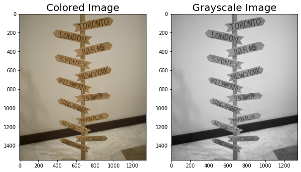
sample = imread('stand.png')
imshow(sample);

sample_g = rgb2gray(sample)
fig, ax = plt.subplots(1,2,figsize=(10,15))
ax[0].imshow(sample)
ax[1].imshow(sample_g,cmap='gray')
ax[0].set_title('Colored Image',fontsize=20)
ax[1].set_title('Grayscale Image',fontsize=20)
plt.show()

To use different morphological operations on the image, we should first binarize the image.

To binarize the image, we can check a sample pixel line value and determine a specific threshold where we will set the pixel value if it's a 0 or 1. Sample checking of pixel values are as follows:

# showing the range of value for a specific y columns
fig, ax = plt.subplots(1,2,figsize=(15,5))

ax[0].set_title('Grayscale Image',fontsize=20)
ax[0].imshow(sample_g,cmap='gray')

ax[1].plot(sample_g[500])
ax[1].set_ylabel('Pixel Value')
ax[1].set_xlabel('Width of Picture')
ax[1].set_title('Plot of 1 Line',fontsize=20)
plt.tight_layout()
plt.show()

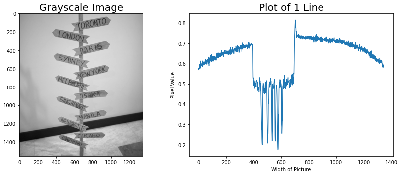
We can see that the sample pixel plotline shows that a majority of the pixel values are above 0.55 while there pixel values that clearly on the lower intensity.

We can also use the mean pixel values of whole images and also the median values of pixel values. Sample and results are as follows:

from scipy import stats
print('Mean Value of Pixels', sample_g.mean())
print('Median Value of Pixels', np.median(sample_g))

Mean Value of Pixels 0.5642273922521608

Median Value of Pixels 0.6111019607843137

med = sample_g.mean()
mea = np.median(sample_g)

med1 = sample_g > med
mea1 = sample_g > mea

fig, ax = plt.subplots(1,3,figsize=(15,5))

ax[0].set_title('Grayscale Image',fontsize=20)
ax[0].imshow(sample_g,cmap='gray')
ax[1].imshow(med1,cmap='gray')
ax[1].set_title('Binarized using Mean Value',fontsize=20)
ax[2].imshow(mea1,cmap='gray')
ax[2].set_title('Binarize using Median Value',fontsize=20)
plt.tight_layout()
plt.show()

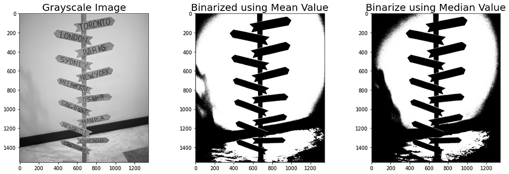
We can see the difference between using the Mean Value and Median Value. It seems that the Mean Value is much more clearer and more distinct rather than the median value.

For now, let us first set a threshold at 0.55 and use the value as the threshold

sample_b = sample_g > 0.55

fig, ax = plt.subplots(1,2,figsize=(10,5))

ax[0].set_title('Grayscale Image',fontsize=20)
ax[0].imshow(sample_g,cmap='gray')
ax[1].imshow(sample_b,cmap='gray')
ax[1].set_title('Binarized Image',fontsize=20)
plt.tight_layout()
plt.show()

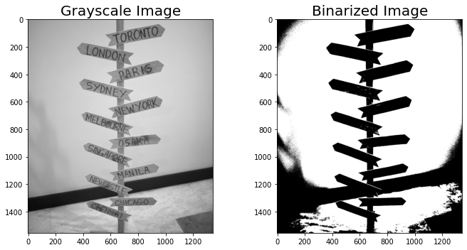
Now that we have a binarized image, we can now perform morphological operations.

Two main kinds of morphing operations are widely used in image processing, they are:

1. Dilation
2. Erosion

Each of this kind has its own effect on the image.

DILATION

In a sense, dilation is the operation where the brightest pixel values of the image are enlarged or made bigger and the darkest pixel values are minimized.

It is easier to visualize it to making the image to be more minimized.

Let us see some examples:

from skimage.morphology import erosion, dilation,opening,closing
selem_ver = np.array([[1,1,1,1,1,1,1,1,1,1,1,1,1,1,1,1,1,1,1,1,1,1,1,1,1,1,1,1,1,1,1,1,
                       0,0,0,0,0,0,0,0,0,0,0,0,0,0,0,0,0,0,0,0,0,0,0,0,0,0,0,0,0,0,0,0,0,0,0,0,0,0,0,
                      1,1,1,1,1,1,1,1,1,1,1,1,1,1,1,1,1,1,1,1,1,1,1,1,1,1,1,1,1,1,1,1,1]])

sample_ver = dilation(sample_b,selem_hor)

fig, ax = plt.subplots(1,3,figsize=(12,5))
ax[0].set_title('Binarized Image',fontsize=15)
ax[0].imshow(sample_b,cmap='gray')
ax[1].imshow(selem_ver,cmap='gray')
ax[1].set_title('Structuring Element',fontsize=15)
ax[2].imshow(sample_ver,cmap='gray')
ax[2].set_title('Morphed Image',fontsize=15)
plt.tight_layout()
plt.show()

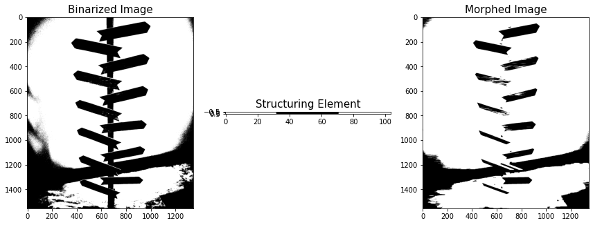
Scikit Library has the nifty function of dilation and erosion where we can feed our binarized image and a structuring element of our choice.

We used a vertical element and feed it to the function to let the image be morphed on the structuring element. From the results, we can see that we were able to take out the vertical features of the images specifically the vertical line depicting the stand.

EROSION

Erosion is the direct opposite of dilation, in erosion we make the images bigger and let the darker pixel values much larger rather than the bright pixel values.

from skimage.morphology import erosion, dilation,opening,closing
selem_ver = np.array([[1,1,1,1,1,1,1,1,1,1,1,1,1,1,1,1,1,1,1,1,1,1,1,1,1,1,1,1,1,1,1,1,
                       0,0,0,0,0,0,0,0,0,0,0,0,0,0,0,0,0,0,0,0,0,0,0,0,0,0,0,0,0,0,0,0,0,0,0,0,0,0,0,
                      1,1,1,1,1,1,1,1,1,1,1,1,1,1,1,1,1,1,1,1,1,1,1,1,1,1,1,1,1,1,1,1,1]])

sample_ver = erosion(sample_b,selem_hor)

fig, ax = plt.subplots(1,3,figsize=(12,5))
ax[0].set_title('Binarized Image',fontsize=15)
ax[0].imshow(sample_b,cmap='gray')
ax[1].imshow(selem_ver,cmap='gray')
ax[1].set_title('Structuring Element',fontsize=15)
ax[2].imshow(sample_ver,cmap='gray')
ax[2].set_title('Morphed Image',fontsize=15)
plt.tight_layout()
plt.show()

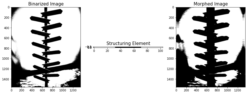
As we can see on the results of the Eroded Image, the whole image was made larger especially the stand in the middle. Notably, the stand grew in size, in reality, what really happened is that the pixel grew in size also covering the other pixels.

Let us try using a different structuring element!

This time a Horizontal Element.

selem_hor = np.zeros((100,5))
selem_hor[0:1]=1
selem_hor[-1:]=1
selem_hor

sample_hor = dilation(sample_b,selem_hor)

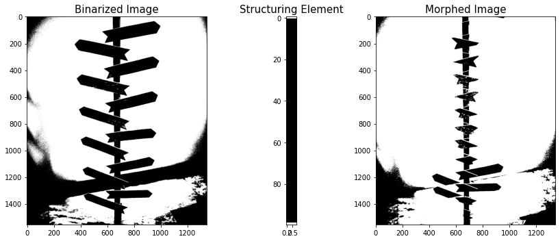
By using a horizontal element, we were to take out the horizontal wood planks in the image without taking out the vertical features of the image.

selem_hor = np.zeros((100,5))
selem_hor[0:1]=1
selem_hor[-1:]=1
selem_hor

sample_hor = erosion(sample_b,selem_hor)

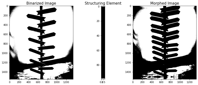
The eroded image as expected grew in size concerning the horizontal axis. It can be noted though that the wood planks in the image multiplied when comparing to the original image.

SUMMARY

We were able to discuss two different morphological operations namely Dilation and Erosion. These two operations are widely used in image processing and used in correcting and completing an image depending on the need of the user. It can be noted also that morphological operations are useful when cleaning very noisy data and also useful in attenuating certain features in an image.

Stay tuned for the next articles!

---

Image Processing using Morphological Operations was originally published in Towards AI on Medium, where people are continuing the conversation by highlighting and responding to this story.

Published via Towards AI