Extracting Features from Text Data

Last Updated on January 6, 2023 by Editorial Team

Author(s): Bala Priya C

Natural Language Processing

Part 3 of the 6 part technical series on NLP

Hey everyone! ? This is part 3 of the 6 part NLP series;

Part 1 of the NLP series introduced basic concepts in Natural Language Processing, ideally NLP101;

Part 2 covered certain linguistic aspects, challenges in preserving semantics, understanding shallow parsing, Named Entity Recognition (NER) and introduction to language models.

In this part, we seek to cover the Bag-of-Words Model and TF-IDF vectorization of text, simple feature extraction techniques that yield numeric representation of the data.?

Understanding Bag-of-Words Model

A Bag-of-Words model (BoW), is a simple way of extracting features from text, representing documents in a corpus in numeric form as vectors.

A bag-of-words is a vector representation of text that describes the occurrence of words in a document.

Why is it called a ‘bag’ ??

It is called a ‘bag’ of words, because any information about the order or contextual occurrence of words in the document is discarded.

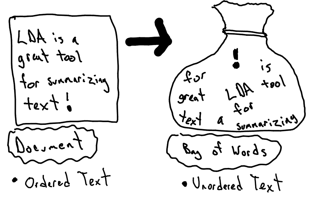
The BoW model only takes into account whether a word occurs in the document, not where in the document. Therefore, it’s analogous to collecting all the words in all the documents across the corpus in a bag 🙂

The Bag-of-Words model requires the following:

• A vocabulary of known words present in the corpus
• A measure of the presence of known words, either number of occurrences/ frequency of occurrence in the entire corpus.

Each text document is represented as a numeric vector, which each dimension denoting a specific word from the corpus. Let’s take a simple example as shown below.

# This is our corpus
It was the best of times,
it was the worst of times,
it was the age of wisdom,
it was the age of foolishness,

Step 1: Collect the data

We have our small corpus, the first few lines from ‘A Tale of Two Cities’ by Charles Dickens. Let’s consider each sentence as a document.

Step 2: Construct the vocabulary

1. Construct a list of all words in the vocabulary
2. Retain only the unique words and ignore case and punctuations (recall: text pre-processing)
3. From the above corpus of 24 words, we now have our vocabulary of 10 words ?

• “it”
• “was”
• “the”
• “best”
• “of”
• “times”
• “worst”
• “age”
• “wisdom”
• “foolishness”

Step 3: Create Document Vectors

As we know the vocabulary has 10 words, we can use a fixed-length document vector of size 10, with one position in the vector to score each word.

The simplest scoring method is to mark the presence of a word as 1, if the word is present in the document, 0 otherwise

Oh yeah! that’s simple enough; Let’s look at our document vectors now! ?

“it was the best of times”  = [1, 1, 1, 1, 1, 1, 0, 0, 0, 0]

“it was the worst of times” = [1, 1, 1, 0, 1, 1, 1, 0, 0, 0]

“it was the age of wisdom”  = [1, 1, 1, 0, 1, 0, 0, 1, 1, 0]

“it was the age of foolishness” = [1, 1, 1, 0, 1, 0, 0, 1, 0, 1]

Guess you’ve already identified the issues with this approach! ‍?‍♀️

• When the size of the vocabulary is large, which is the case when we’re dealing with a larger corpus, this approach would be a bit too tedious.
• The document vectors would be of very large length, and would be predominantly sparse, and computational efficiency is clearly suboptimal.
• As order is not preserved, context and meaning are not preserved either.
• As the Bag of Words model doesn’t consider order of words, how can we account for phrases or collection of words that occur together?

Do you remember the N-grams language model from part 2??

Oh yeah, a straight forward extension of Bag-of -Words to Bag-of-N-grams helps us achieve just that!

An N-gram is basically a collection of word tokens from a text document such that these tokens are contiguous and occur in a sequence. Bi-grams indicate n-grams of order 2 (two words), Tri-grams indicate n-grams of order 3 (three words), and so on.

The Bag of N-Grams model is hence just an extension of the Bag of Words model so we can also leverage N-gram based features.

• This method does not take into account the relative importance of words in the text. ?

Just because a word appears frequently, does it necessarily mean it’s important ? Well, not necessarily.

In the next section, we shall look at another metric, the TF-IDF score, which does not consider ordering of words, but aims at capturing the relative importance of words across documents in a corpus.

Term Frequency- Inverse Document Frequency

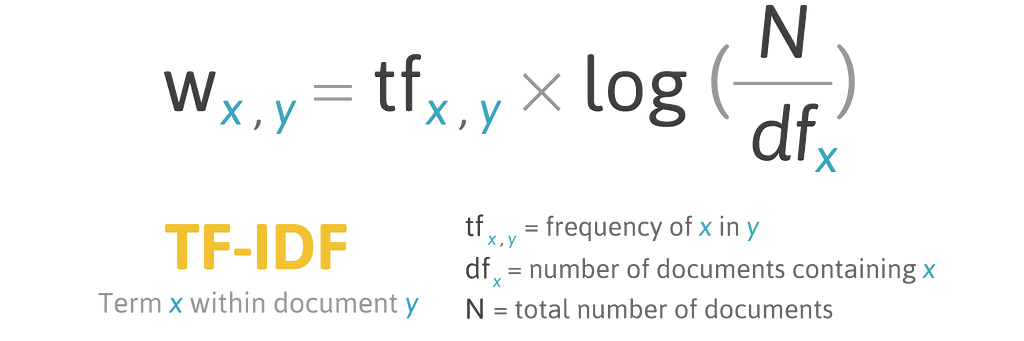
Term Frequency- Inverse Document Frequency (TF-IDF Score) is a combination of two metrics — the Term Frequency (TF) and the Inverse Document Frequency (IDF)

The idea behind TF-IDF score which is computed using the formula described below is as follows:

“ If a word occurs frequently in a specific document, then it’s important whereas a word which occurs frequently across all documents in the corpus should be down-weighted to be able to get the words which are actually important.”

Here’s another widely used formula;

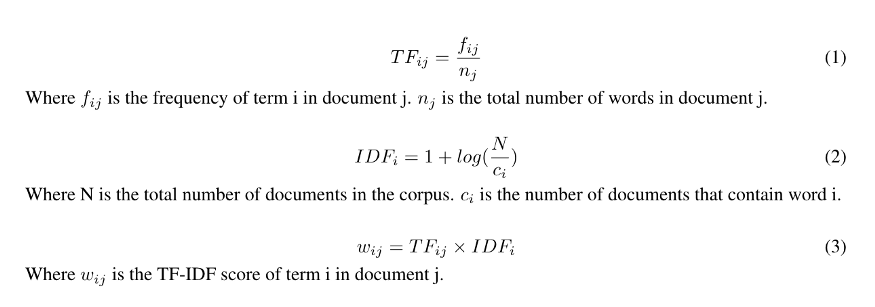
The above formula helps us calculate the TF-IDF score for term i in document j and we do it for all terms in all documents in the corpus. We therefore, get the term-document matrix of shape num_terms x num_documents . Here’s an example.

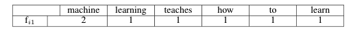
Document 1: Machine learning teaches machine how to learn

Document 2: Machine translation is my favorite subject

Document 3: Term frequency and inverse document frequency is important

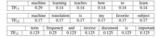
Step 1: Computing f_{ij}; Frequency of term i in document j

For Document 1:

For Document 2:

For Document 3:

Step 2: Computing Normalized Term Frequency

As shown in the above formula, the f_{ij} obtained above should be divided by the total number of words in document j .

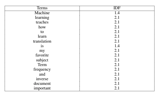
Step 3: Compute Inverse Document Frequency (IDF) score for each term

Step 4: Obtain the TF-IDF Scores

Now that we’ve calculated TF_{ij} and IDF_{ij}, let’s go ahead and multiply them to get the weights w_{ij} (TF-IDF_{ij}).

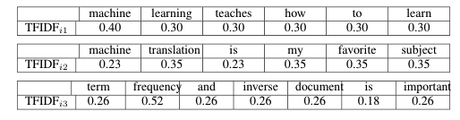
Starting with raw text data, we’ve successfully represented the documents in numeric form. Oh yeah! We did it!?

Now that we know to build numeric features from text data, as a next step, we can use these numeric representations to understand tutorials on understanding document similarity, similarity based clustering of documents in a corpus and generating topic models that are representative of latent topics in a large text corpus.

So far, we’ve looked at traditional methods in Natural language Processing. In the next part, we shall take baby steps into the realm of Deep learning for NLP.✨

Happy learning! Until next time ?

References

Here’s the link to the recording of the webinar.

---

Extracting Features from Text Data was originally published in Towards AI on Medium, where people are continuing the conversation by highlighting and responding to this story.

Published via Towards AI