Convolution of Signals in 1-Dimension

Last Updated on May 22, 2020 by Editorial Team

Author(s): sinchana S.R

Mathematics

Convolution is one of the most useful operators that finds its application in science, engineering, and mathematics

Convolution is a mathematical operation on two functions (f and g) that produces a third function expressing how the shape of one is modified by the other.

Convolution of discrete-time signals

A simple way to find the convolution of discrete-time signals is as shown

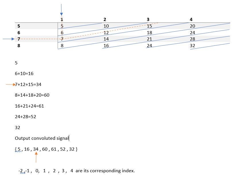
Input sequence x[n] = {1,2,3,4} with its index as {0,1,2,3}

Impulse response h[n] = {5,6,7,8} with its index as {-2,-1,0,1}

The blue arrow indicates the zeroth index position of x[n] and h[n]. The red pointer indicates the zeroth index position of the output convolved index. We can construct a table, as shown below. Multiply the elements of x and h as shown, and add them up diagonally.

>> clc;  % clears the command window
>> clear all; % clears all the variables in the workspace
>> close all; % closes all the figure window

Taking the input from the user

>> % x[n] is the input discrete signal.
>> x=input('Enter the input sequence x =');
>> nx=input('Enter the index of the input sequence nx=');
>> % h[n] is the impulse response of the system.
>>h=input('Enter the impulse response of the system,second sequence h=');
>> nh=input('Enter the index of the second sequence nh=');

The output in the command window,

Enter the input sequence x =[1 2 3 4]
Enter the index of the input sequence nx=[0 1 2 3]
Enter the impulse response of the system,second sequence h=[5 6 7 8]
Enter the index of the second sequence nh=[-2 -1 0 1]

Calculating the index of the convolved signal,

>> % Index of the convolved signal
>> n=min(nx)+min(nh):max(nx)+max(nh);

Convolution

>> y=conv(x,h);

Display

>> disp('The convolved signal is:');
>> y
>> disp('The index of convolved sequence is:');
>> n

The output in the command window,

>> The convolved signal is:

y =

5    16    34    60    61    52    32

>> The index of convolved sequence is:

n =

-2    -1     0     1     2     3     4

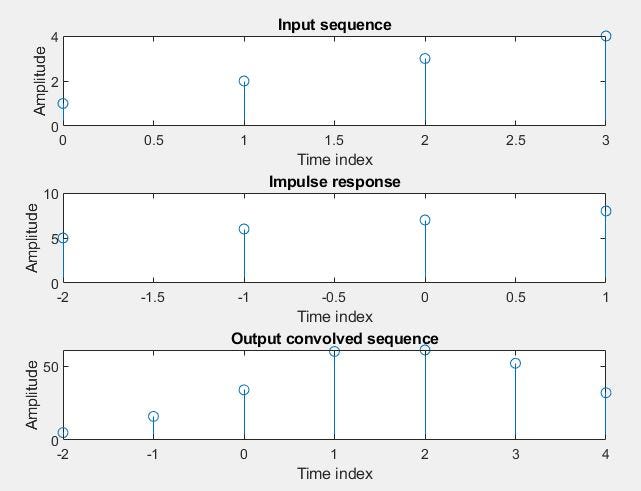
Let’s visualize these signals.

>> subplot(311);
>> stem(nx,x);
>> subplot(312);
>> stem(nh,h);
>> subplot(313);
>> stem(n,y);

You can find the code on Github.

Convolution of continuous-time signals

>> clc;
>> clear all;
>> close all;
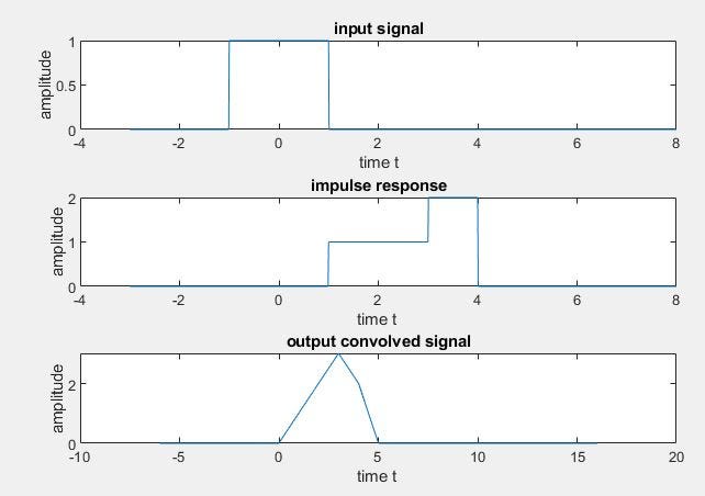
>> t=-3:0.01:8;
>> x=(t>=-1 & t<=1); % pulse that exists for t>=-1 and t<=1
>> subplot(311);
>> plot(t,x);
>> h1=(t>=1 & t<=3); % pulse that exists for t>=1 & t<=3
>> h2=(t>3 & t<=4); % pulse that exists for t>3 & t<=4
>> h=h1+(2*h2);
>> subplot(312);
>> plot(t,h);
>> y=convn(x,h);
>> y=y/100;
>> t1=2*min(t):0.01:2*max(t);
>> subplot(313);
>> plot(t1,y);

You can find code on Github.

Properties of Convolution

Convolution is a linear operator and has the following properties.

• The Commutative Property

x[n] * h[n] = h[n] * x[n] ( in discrete time )

x(t) * h(t) = h(t) * x(t) ( in continuous time )

• The Associative Property

x[n] * (h1[n] * h2[n]) = (x[n] * h1[n]) * h2[n] ( in discrete time )

x(t) * (h1(t) * h2(t)) = (x(t) * h1(t)) * h2(t) ( in discrete time )

• The Distributive Property

x[n] * (h1[n] + h2[n]) = (x[n] * h1[n]) + (x[n] * h2[n]) ( in discrete time )

x(t) * (h1(t) + h2(t)) = (x(t) * h1(t)) + (x(t) * h2(t)) ( in discrete time )

• Associativity with scalar multiplication

a(f * g) = (af) * g

for any real (or complex) number a

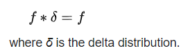
• Multiplicative identity

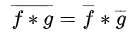
• Complex conjugation

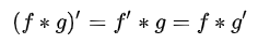
• Relationship with differentiation

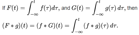
• Relationship with integration

Applications

Convolution finds its applications in many domains including digital image processing, digital signal processing, optics, neural networks, digital data processing, statistics, engineering, probability theory, acoustics, and many more.

References

• Signals and Systems by Oppenheim and Willsky, Second edition.
• https://en.wikipedia.org/wiki/Convolution

---

Convolution of Signals in 1-Dimension was originally published in Towards AI — Multidisciplinary Science Journal on Medium, where people are continuing the conversation by highlighting and responding to this story.

Published via Towards AI