


YouTube Dislikes Prediction in Real-time — Working With a Combination of Data; A Practical Guide
Last Updated on July 17, 2023 by Editorial Team
Author(s): Nafiu
Originally published on Towards AI.
Hi everyone, this is a practical guide to a fascinating topic; today, we will discuss how you can work with a combination of mixed data. Well, we have all gone through it when we go through a dataset, and there are features with different data types and wonder how we can combine both types and use them for training a single machine learning model. Well, today, you have the simple guided answer for that. Also, to make things interesting, we will train a machine-learning model that predicts youtube dislikes in real-time. It's no surprise anymore that youtube removed its dislike count feature a year ago, maybe I’m even a little late to solve this problem, but the dataset we are using today is for sure gonna fulfill our needs of learning for today. Remember that since youtube dislike is a number, we are solving a regression problem. U+1F642
Table of contents
What you will learn
- Work with mixed data
- Clean text data
- Process both text and numeric data
- Keras TensorFlow functional API
- LSTM (RNN)
- To create a model that processes different types of data at once
- how to check the accuracy of a regression model
- Youtube API
Reality: in youtube, the amount of views, likes, and dislikes that a video can get depends on a lot of things, such as the popularity of the creator, the quality of the video, SEO, user shares, and a lot of other thighs which goes beyond the dataset available for us. Anyways let’s try to get the best out of what we have U+1F601
Note: throughout this tutorial, I will be mentioning what and how you can do to improve this model and the things I have missed while creating this if I missed anything. And when it comes to adding libraries, we will be adding as we need instead of importing all of them once
Let’s get started…
You can get the dataset at https://www.kaggle.com/datasets/dmitrynikolaev/youtube-dislikes-dataset
Please download the dataset and extract it in your working directory. This dataset is a mixed language dataset of 37422 unique raws we are gonna shorten it down to only English language by using the video ids provided with the dataset, which makes our dataset 15835 unique raws in total before processing. This is actually a very short amount of data to solve a problem like this, try to increase the amount of data by processing other languages, too which will surely help to increase model accuracy.
Note: This dataset was last updated on 13/12/2021 so we will assume that is the date that this data was extracted since we will use this data to deal with the time period
Load the dataset and collect the features we need
Hope you have the .csv file in your working directory, well let’s load it using pandas and shorten it down to only English and get more details of the available features from the dataset.
Import some libraries to get started
import numpy as np
import pandas as pd
import tensorflow as tf
Loading the dataset
dataset = pd.read_csv('youtube_dislike_dataset.csv')
dataset.head()
Collecting only English data
file_US_ids = open("video_IDs/unique_ids_US.txt", "r")
US_ids = file_US_ids.read().splitlines()
dataset = dataset[dataset['video_id'].isin(US_ids)]
dataset.shape
Checking more details of the dataset, such as the data types of the features
dataset.info()
The dataset contains 12 features. We only will use 7 features from these. These features are described below:
Video_id: unique video id
Title: title of the youtube video
Channel_id: channel id of the publisher
Channel_title: name of the channel
Published_at: the date that the video was published
View_count: Number of views that video got in a period of time
Likes: Number of likes that video has
Dislikes: Number of dislikes that video got in a period of time
Comment_count: Number of comments that the video has
Tags: video tags as strings
Description: Video description
Comments: list of video comments as a string
Well, there you have all the features available, now let’s select some of them which we will use in this practical guide.
We will be using the following 7 features:
view_count, published_at, likes, comment_count, tags, description, dislikes
dataset = dataset[['view_count', 'published_at','likes', 'comment_count','tags','description','dislikes']]
We will create one more feature and also will get rid of one feature from here in the pre-processing stage. Honestly, using the title and channel name would be a great improvement for the model, you can try it. U+1F642
Data pre-processing
Let’s get started with processing data, in this stage, we do a lot of important things to our datasets such as dealing with missing values, creating related time fields, and cleaning and tokenizing text data. Let me explain more while doing it.
Dealing with missing values
The dataset is quite tricky if you just look for missing values (nan) you will not find anything this is because in a way the dataset doesn’t have any missing values since all the fields are filled with an empty string, so handle this case we will check for empty strings fields that don’t have a word in it and convert it into a nan value and check again, I’m sure we will get a good amount of null values now. And guess what? We will drop them all, this will make our dataset shot to 13536 raws in total, which is pretty small U+1F602

Creating a new feature — dealing with time
Above, I mention that we are going to assume that the data was extracted on 13/12/2021, well, this is the time that date comes into play.
We are gonna create a new feature named timesec by calculating the amount of time between the date that the video was published and the time it was extracted in minutes.
So basically: timesec = extracted date – published_at date
First, we will write a function to calculate the time between two points in minutes and use the pandas apply method to create the new feature.
Function to calculate the time between:
from datetime import datetime
def calTime(time):
 start = datetime.strptime(time, '%Y-%m-%d %H:%M:%S')
 end = datetime.strptime('13/12/2021 00:00:00', '%d/%m/%Y %H:%M:%S') # assuming this is the date that this dataset was extracted
 return np.round((end - start).total_seconds() / 60, 2)
Using pandas apply method to run the function and create the new feature
dataset['timesec'] = dataset['published_at'].apply(calTime)
Cleaning the text features
We will create a function to clean our text data followed by a set of steps that will get the right and important meaning out of it.
Basically, the function will remove any unnecessary URLs, punctuation marks, numbers, stopwords, and random words that are not in the dictionary will be removed. It will also deal with contractions words and will lemmatize words and at last, will convert all to lowercase and return the processed string. We will do this with help of a bunch of libraries so let’s get started by importing those.
Importing the required libraries for this
import re
from string import punctuation
from bs4 import BeautifulSoup
import nltk
nltk.download('stopwords')
nltk.download('wordnet')
nltk.download('omw-1.4')
nltk.download('words')

from nltk.corpus import stopwords
from nltk.stem import WordNetLemmatizer
The contraction word dictionary will help to convert a combination of two words to their separate root word. (this is not all, there are more)
contraction_map={
 "ain't": "is not",
 "aren't": "are not",
 "can't": "cannot",
...
}
The function we created to clean text
lemmatizer = WordNetLemmatizer()
in_words = set(nltk.corpus.words.words())
def clean_text(text):
 text = str(text)
 text = BeautifulSoup(text, "lxml").text
 text = re.sub(r'\([^)]*\)', '', text)
 text = re.sub('"','', text)
 text = ' '.join([contraction_map[t] if t in contraction_map else t for t in text.split(" ")])
 text = re.sub(r"'s\b","",text)
 text = re.sub("[^a-zA-Z]", " ", text)
 text = " ".join(w for w in nltk.wordpunct_tokenize(text) if w.lower() in in_words or not w.isalpha())

 text = [word for word in text.split( ) if word not in stopwords.words('english')]
 text = [lemmatizer.lemmatize(word) for word in text]
 text = " ".join(text)
 text = text.lower()
 return text
At last creating two new columns with cleaned text after running the function
%time dataset['clean_description'] = dataset['description'].apply(clean_text)
%time dataset['clean_tags'] = dataset['tags'].apply(clean_text)
Splitting data
Since we are using different datatypes it's not ideal to use the usual train_test_split function so we will start by splitting data by train and test with the help of slicing after that we will separate X and Y from both train and test data, then will separate the text and numerical features, we will keep both tags and description separate but will keep all the numeric features as one. This might be confusing anyway let’s see the code, which will make things clear.
Note: Y is the dislike feature and our target variable. And X would be the view_count, likes, comment_count, timesec, clean_tags, clean_description. We don’t need the published_at feature.
Slicing to train and test
# Slicing to train and test
dataset_train = dataset.iloc[:12500,:]
dataset_test = dataset.iloc[12501:,:]

# Creating X and Y variables of train dataset
X_train = dataset_train.loc[:, dataset.columns != 'dislikes']
Y_train = dataset_train['dislikes'].values

#Creating X and Y variables of the test dataset
X_test = dataset_test.loc[:, dataset.columns != 'dislikes']
Y_test = dataset_test['dislikes'].values

# Splitting and organizing the features of train data
X_train_numaric = X_train[['view_count', 'likes', 'comment_count', 'timesec']].values
X_train_tags = X_train['clean_tags'].values
X_train_desc = X_train['clean_description'].values

# Splitting and organizing the features of the test data
X_test_numaric = X_test[['view_count', 'likes', 'comment_count', 'timesec']].values
X_test_tags = X_test['clean_tags'].values
X_test_desc = X_test['clean_description'].values
Text tokenization — processing text
Here we are gonna create a function to tokenization function to process our text features. The function will create a tokenizer and tokenize words and will add padding of 100 to it and will return a set of useful information such as processed test and train data, the number of max words, the vocabulary and the size of it, and the tokenizer itself that we will use later to make real-time predictions.
We will have to use this on both tags and description features as well.
Let’s get to the code. U+1F642
Importing required libraries for this
from tensorflow.keras.preprocessing.text import Tokenizer
from tensorflow.keras.preprocessing.sequence import pad_sequences
The function to do the processing
def Tokenizer_func(train,test, max_words_length=0, max_seq_len=100):
 tokenizer = Tokenizer()
 tokenizer.fit_on_texts(train)

 max_words = 0
 if max_words_length > 0:
 max_words = max_words_length
 else:
 max_words = len(tokenizer.word_counts.items())

 tokenizer = Tokenizer(num_words=max_words)
 tokenizer.fit_on_texts(train)

 train_sequences = tokenizer.texts_to_sequences(train)
 test_sequences = tokenizer.texts_to_sequences(test)

 train = pad_sequences(train_sequences,maxlen=max_seq_len, padding='post')
 test = pad_sequences(test_sequences,maxlen=max_seq_len, padding='post')

 voc = tokenizer.num_words +1
 return {'train': train, 'test': test, 'voc': voc, 'max_words':max_words, 'tokenizer': tokenizer}
Calling the function for tags
X_tags_processed = Tokenizer_func(X_train_tags,X_test_tags)
# Extracting data from it…
X_train_tags,X_test_tags,x_tags_voc,x_tags_max_words,x_tag_tok = X_tags_processed['train'], X_tags_processed['test'],X_tags_processed['voc'],X_tags_processed['max_words'],X_tags_processed['tokenizer']
Calling the function for description
X_desc_processed = Tokenizer_func(X_train_desc,X_test_desc)
# Extracting data from it…
X_train_desc, X_test_desc,x_desc_voc,x_desc_max_words,x_desc_tok = X_desc_processed['train'], X_desc_processed['test'],X_desc_processed['voc'],X_desc_processed['max_words'],X_desc_processed['tokenizer']
Well, we have one more thing to do before ending the processing step of this tutorial.
Numeric data normalization
For this, we will use the StandardScaler to normalize both train and test data. Well, let’s see the code.
Importing the libraries, Creating the Scaler, and processing numeric data using it
from sklearn.preprocessing import StandardScaler
Sc = StandardScaler()
X_train_numaric = Sc.fit_transform(X_train_numaric)
X_test_numaric = Sc.transform(X_test_numaric)
Yay.. we are halfway done… this is the end of data preprocessing. U+1F389U+1F389U+1F389
Creating the Model and Training
Here we will be using Keras functional API to create a machine-learning model we will be building a type of an RNN known as LSTM to process text data and later connected it to an MLP with the numeric data. I’m not gonna explain LSTM here since I have already gone through it in a previous post which is linked here…
Stock market prediction using LSTM; will the price go up tomorrow. Practical guide
The goal of this tutorial is to create a machine learning model to predict the future value of a stock traded on a…
medium.com
Allow me to explain our model here:
We have 3 inputs in the model: tags input, description input which has an input shape of none, and numeric which has an input size of 4 since we have 4 numeric features. Both tags and description starts with an embedding layer and then with two LSTM layer with units of 100 (remeber we added 100 as padding) followed by a normalization layer after each LSTM later. For both features, the first LSTM layer will have a dropout of 0.2 and return sequence set to true, and the second layer comes with a dropout of 0.4 and return sequence set to false. After passing through those layers both tags and description are combined with numeric data input and then passed through 4 dense layers with the units of 256,128,32, and 1, the first 3 layers with relu activation function and the last layer with a linear activation function (coz the problem is regression). Next, the whole model is compiled using model.compile() method, set as mean_squared_error as a loss function and mean_absolute_error as a matric and adam as an optimizer, as adam functions learning rate decreased to 0.001. Then finally we can view the summary of the model by using model.summary() method.
Let's view the code…
Import required libraries for this.
from keras.models import Model
from tensorflow.keras.layers import Input, LSTM, Embedding, Dense, concatenate,LayerNormalization
from keras.optimizers import Adam
from keras.callbacks import EarlyStopping
Creating the model
tagsInput = Input(shape=(None,), name='tags')
descInput = Input(shape=(None,), name='desc')
numaricInput = Input(shape=(4,), name='numaric')

tags = Embedding(input_dim=x_tags_voc,output_dim=8,input_length=x_tags_max_words)(tagsInput)
tags = LSTM(100,dropout=0.2, return_sequences=True)(tags)
tags = LayerNormalization()(tags)
tags = LSTM(100,dropout=0.4, return_sequences=False)(tags)
tags = LayerNormalization()(tags)

desc = Embedding(input_dim=x_desc_voc,output_dim=8,input_length=x_desc_max_words)(descInput)
desc = LSTM(100,dropout=0.2, return_sequences=True)(desc)
desc = LayerNormalization()(desc)
desc = LSTM(100,dropout=0.4, return_sequences=False)(desc)
desc = LayerNormalization()(desc)

combined = concatenate([tags, desc,numaricInput])
x = Dense(256,activation='relu')(combined)
x = Dense(128,activation='relu')(x)
x = Dense(32,activation='relu')(x)
x = Dense(1,use_bias=True,activation='linear')(x)
model = Model([tagsInput, descInput,numaricInput], x)
Compiling the model
model.compile(loss='mean_squared_error', optimizer=Adam(learning_rate=0.001, decay=0.001 / 20), metrics=['mae'])
Now let's see the summary of the model using model.sumary() method
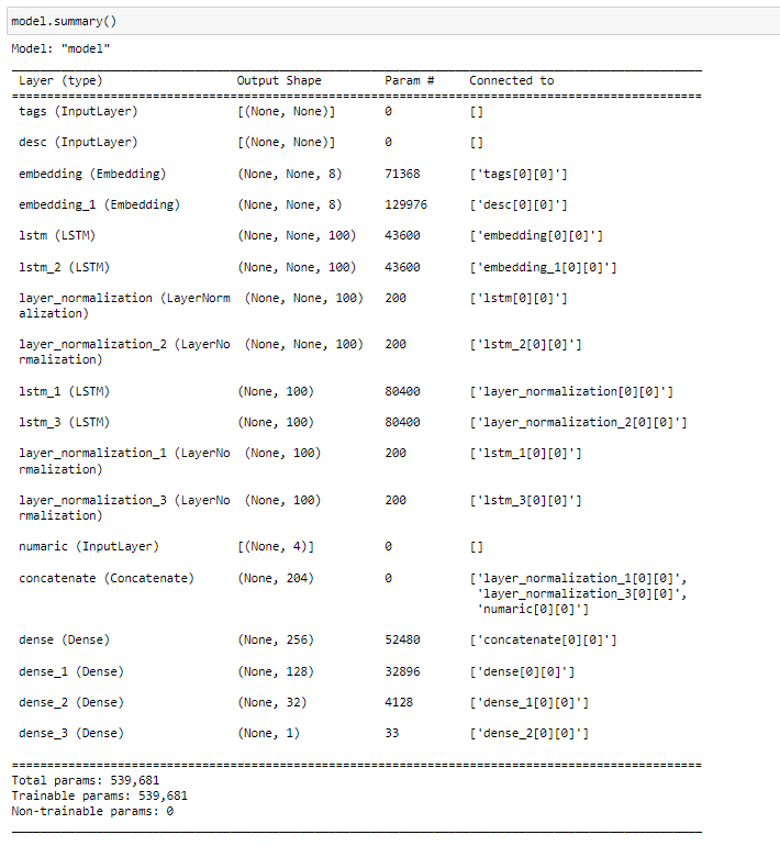
Now it's time to train our model. We will train our model under 500 epochs with a batch size of 25 and with a validation split of 2 percent, since we have the early stopping on it will probably be done training the model before it even comes close to 500 epochs.
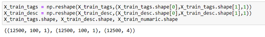
Well, there is one more thing that we must do before starting to train our model. LSTM supports 3-dimensional data but our data is 2 dimensional so we must convert it into 3-dimensional data before we start training
Initializing EarlyStopping to avoid overfitting while training the model
es = EarlyStopping(monitor='val_loss', mode='min', verbose=1, patience=20)
Reshaping the data to 3-dimensional data
X_train_tags = np.reshape(X_train_tags,(X_train_tags.shape[0],X_train_tags.shape[1],1))
X_train_desc = np.reshape(X_train_desc,(X_train_desc.shape[0],X_train_desc.shape[1],1))
X_train_tags.shape, X_train_desc.shape, X_train_numaric.shape
Training the model
history = model.fit(
 x=[X_train_tags, X_train_desc,X_train_numaric],
 y=Y_train,
 epochs=500,
 batch_size=25,
 validation_split=0.2,
 verbose=1,
 callbacks=[es]
 )

Here we can see our model has stopped training once it reaches 26 epochs.
Evaluating our model
Now that our model has done training, it’s time to check the results but before that, let’s answer a simple question and understand a couple of important things.
How to check the accuracy of a regression model?
Residuals — The difference between the predicted value and the actual value.
Mean Absolute Error — the mean value of the residuals between predicted values and actual values.
- The lower the MAE the better the model is.
- MAE is calculated by adding residuals and dividing by the length of the dataset (test data)
- Describes how close the predictions are to the actual values on average.
Mean Squared Error — shows how close a regression line is to a set of data points
Root Mean Squared Error — is the square root of the mean of all the squared values of errors
- indicates the absolute fit of the model relative to the given data
- RMSE has a relationship with MAE
- If RMSE value is much higher than MAE, it means the results of some large errors in the dataset.
R-squared — shows how well the data fits into the model
- Outputs a value on a scale of 0 to 1
- The higher the R2 the better the model is
- R2 score value can be used to get the accuracy of the model same as a classification model by multiplying the value * 100
Key points:
- R2 must be high
- The lower MSE the better the model is
- The lower MAE the better the model is
- The lower RMSE the better the model is
- MAE should be lower then RMSE
Now let’s implement these in our project and see the model results. We can do this by using the following code
pprydd = model.predict([X_test_tags, X_test_desc, X_test_numaric])
from sklearn import metrics
print("Mean Absolute Error (MAE) - Test data : ", metrics.mean_absolute_error(Y_test, pprydd))
print("Mean Squared Error (MSE) - Test data : ", metrics.mean_squared_error(Y_test, pprydd))
print("Root Mean Squared Error (RMSE) - Test data : ", np.sqrt(metrics.mean_squared_error(Y_test, pprydd)))
print("Co-efficient of determination (R2 Score): ", metrics.r2_score(Y_test, pprydd))
We can see that our model has an R2 score of 0.82 (82%) but also, we can see we have a very high MSE which is not a good sign U+1F625. And we can see both MAE and RMSE are pretty low compared to MSE, which is fine but the RMSE is higher than the MAE, which actually indicates the result of some errors in our dataset U+1F915… not the best model in the world but in my opinion, this is not bad compare to the usable data we had.
Note: you can try improving the model by doing more research about this field, like what are the things that depend on while getting more dislike on videos and focus on that. Also, try using the features that we didn’t use in this tutorial… anyways, leys continue.
Real-time prediction
Now, the part we all have been waiting for to predict youtube dislike in real-time. For this, we will be using youtube API to get targeted video data by id and collect the required data from it and process it and run it through the model. To make things easy, we will write a function to make this all happen at once.
Let’s see the code. 🙂
Import the required library
import googleapiclient.discovery
Create youtube client
DEVELOPER_KEY = 'YOUR_API_KEY'
youtube_client = googleapiclient.discovery.build('youtube', 'v3', developerKey=DEVELOPER_KEY)
Time to write the function. Let me explain how this works.
Once the data is received, we will extract the required fields from it
For both text fields, the text will be cleaned using the previously created cleaning function and then will be processed through the tokenizer we created earlier, and at last, the padding will be added to the text.
The timesec field will be calculated using the next function. Inside this function, it will get the time period between the date that the targeted video was published and today in minutes.
Next, all the numeric features will be passed through the Scaler for normalization. Once the processing is done, then we will predict the dislike of the video by passing through the model, and the function will return the predicted dislike number among some other useful information.
def realtime(youtube,video_id):
 def calTimesss(time):
 start = datetime.strptime(time, '%Y-%m-%dT%H:%M:%S%z')
 end = datetime.now()
 return np.round((end - start.replace(tzinfo=end.tzinfo)).total_seconds() / 60, 2)
 request = youtube.videos().list(part="snippet, statistics",id=video_id)
 response = request.execute()

 desc = response['items'][0]['snippet']['description']
 desc =[clean_text(desc)]
 desc = x_desc_tok.texts_to_sequences(desc)
 desc = pad_sequences(desc,maxlen=100, padding='post')

 tags = response['items'][0]['snippet']['tags']
 tags=(" ".join(tags))
 tags =[clean_text(tags)]
 tags = x_tag_tok.texts_to_sequences(tags)
 tags = pad_sequences(tags,maxlen=100, padding='post')

 publishedAt = response['items'][0]['snippet']['publishedAt']
 timesec = calTimesss(publishedAt)
 viewcount = response['items'][0]['statistics']['viewCount']
 likeCount = response['items'][0]['statistics']['likeCount']
 commentCount = response['items'][0]['statistics']['commentCount']
 numaricdata = [[viewcount, likeCount,commentCount,timesec]]
 numaricdata = Sc.transform(numaricdata)

 pryd = model.predict([tags, desc, numaricdata])

 return {"predicted": int(pryd[0][0]), "info": {
 "video_id": video_id,
 "likes": likeCount,
 "commentCount": commentCount,
 "viewCount": viewcount,
 "publishedAt": publishedAt,
 "dislike": int(pryd[0][0]),
 }}
Now let's run it, and let’s see the results…
video_id = "videoid"
realtime(youtube_client, video_id)
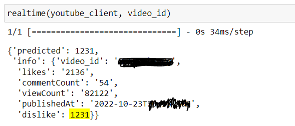
Haha, it worked U+1F602 U+1F389. According to the model, this video has 1231 diskiles. Ouch, a lot of haters U+1F61F
Well, this is the end of this tutorial about working with combination data, it was fun so hope you enjoyed it. Also hope you will try to improve this model… Keep learning U+1F642
link to GitHub repo: https://github.com/nafiu-dev/youtube_dislike_prediction_practice
you can connect with me here:
https://www.instagram.com/nafiu.dev
Linkedin: https://www.linkedin.com/in/nafiu-nizar-93a16720b
My other posts:
End to End full stack project from backend, frontend and machine learning to ethical hacking…
Hi, I welcome you all to this series of building an end to end project starting from backend development, front-end…
medium.com
Create a Boolean Image Classifier Fast With Any Data Set, With a Brief Explanation of the…
Hi everyone, in this post, we are going to look at a type of neural network called the Convolutional Neural Network…
pub.towardsai.net
Highlighting the most popular machine learning algorithms; Implementing it
Overview of the most popular machine learning models, implementing and comparing the accuracy using iris dataset
medium.com
Join thousands of data leaders on the AI newsletter. Join over 80,000 subscribers and keep up to date with the latest developments in AI. From research to projects and ideas. If you are building an AI startup, an AI-related product, or a service, we invite you to consider becoming a sponsor.
Published via Towards AI
Related posts


Popular posts

 for 2021")


Updates

Recent Posts


