


Unlocking the Power of Concave and Convex Functions in Machine Learning
Last Updated on July 25, 2023 by Editorial Team
Author(s): Towards AI Editorial Team
Originally published on Towards AI.
A Comprehensive Introduction for Beginners
Author(s): Pratik Shukla
“Courage is never to let your actions be influenced by your fears.” — Arthur Koestler
Table of Contents:
- Why do we care so much about whether a function is convex or concave?
- What is a concave and convex function?
- Algebraic proof of concavity
- Algebraic proof of convexity
- Visual proof of a convex function with an example
- Visual proof of a concave function with an example
- Conclusion
- Resources and References
Introduction:
Concave and convex functions are an important concept in mathematics and are widely used in various fields, including economics, optimization, and machine learning. Understanding the properties and behavior of these functions is crucial for solving optimization problems, making predictions, and making informed decisions. However, the topic of concave and convex functions can be challenging for many people due to its abstract nature and the complexity of the mathematical concepts involved. In this blog, we will provide a not-so-gentle introduction to concave and convex functions that will help you gain a better understanding of their properties and behavior. We will cover the basics of concavity and convexity, the differences between the two, and their implications in real-world applications. By the end of this blog, you will have a solid foundation on concave and convex functions, which will serve as a steppingstone to further exploring this fascinating topic.
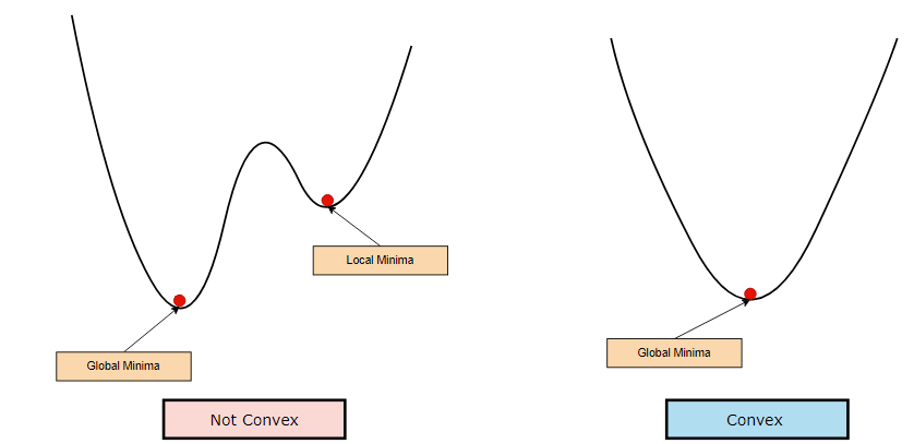
Why do we care so much about whether a function is concave or convex?
While performing classification, we usually use a gradient-based technique to find the optimal values of the coefficients by minimizing the loss function. From the below graphs, we can say that if the function is not convex then it is not guaranteed that we will reach the global minima. In the case of non-convex functions, there is a possibility that we will be stuck at local minima. To avoid this problem, we prefer that our loss function is convex when we are using the gradient descent algorithm.
What is a concave and convex function?
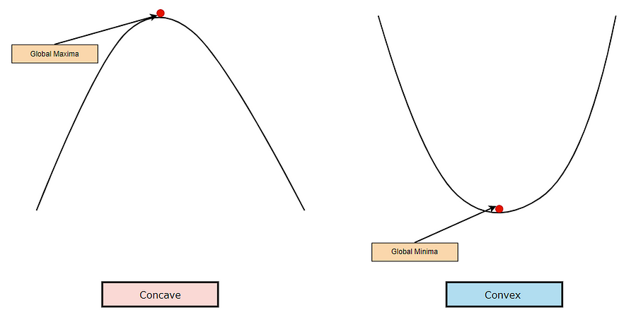
1. Concave Function:
A function of a single variable is called a concave function if no line segments joining two points on the graph lie above the graph at any point.
2. Convex Function:
A function of a single variable is called a convex function if no line segments joining two points on the graph lie below the graph at any point.
3. Neither Concave nor Convex:
A function of a single variable is neither a convex nor a concave function if the line segments lie above the graph at some points and below the graph at some points.
How to check whether a function is concave or convex?
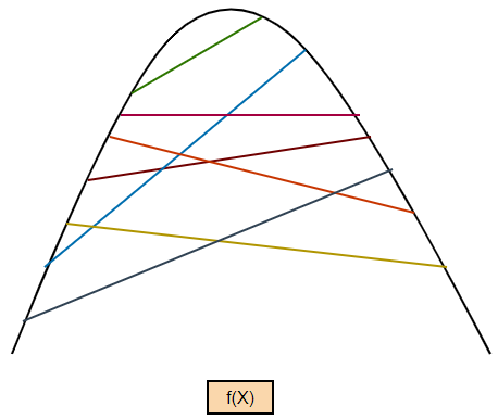
1. Algebraic proof of concavity:
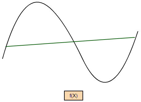
Let’s say f(u) is a function defined on the interval [a, b]. According to the definition, this function is concave if, for every pair of numbers X and Y with the condition a ≤ X ≤ b and a ≤ Y ≤ b, the line segment from (X, f(X)) to (Y, f(Y)) lies on or below the graph of the function. This is clearly illustrated in the following diagram. Now, let’s prove it algebraically!

1. Step — 1:
The function f(u) is defined over the interval [a, b].
2. Step — 2:
Let’s take two points X and Y such that a ≤ X ≤ b and a ≤ Y ≤ b. The corresponding points on the vertical axis can be denoted by f(X) and f(Y) respectively.
3. Step — 3:
Any point P between [X, Y] can be written as follows.

Here, 0 ≤ λ ≤ 1. If λ=0, then P=Y. If λ=1 then P=X.
4. Step — 4:
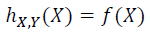
Next, draw a straight line connecting (X, f(X)) and (Y, f(Y)). Now, let’s say the height of the line segment from (X, f(X)) to (Y, f(Y)) at any point P (X ≤ P ≤ Y) is given by,

5. Step — 5:
Based on this, we can say that the height of the line segment from (X, f(X)) to (Y, f(Y)) at point X will be…
Similarly, we can say that the height of the line segment from (X, f(X)) to (Y, f(Y)) at point Y will be…

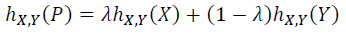
6. Step — 6:
Based on this, we can say that the height of the line segment from (X, f(X)) to (Y, f(Y)) at point P will be…

7. Step — 7:
Next, we are simplifying the equation in Step — 6.
8. Step — 8:
Next, we are substituting the values of Step — 5 into Step — 7.


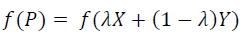
9. Step — 9:
Next, we can define the value of f(P) as…
10. Step — 10:
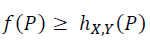
According to the definition of a concave function, the function f is concave if and only if for every pair of numbers X and Y with a ≤ X ≤ b and a ≤ Y ≤ b, we have…
11. Step — 11:

The above condition must be true for every value 0≤ λ ≤1.
In conclusion, we can say that a function is concave when the above condition is met.
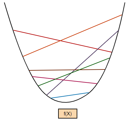
2. Algebraic proof of convexity:
Let’s say f(u) is a function defined on the interval [a, b]. According to the definition, this function is convex if, for every pair of numbers X and Y with the condition a ≤ X ≤ y and a ≤ Y ≤ b, the line segment from (X, f(X)) to (Y, f(Y)) lies on or above the graph of the function. This is clearly illustrated in the following diagram. Now, let’s prove it algebraically!
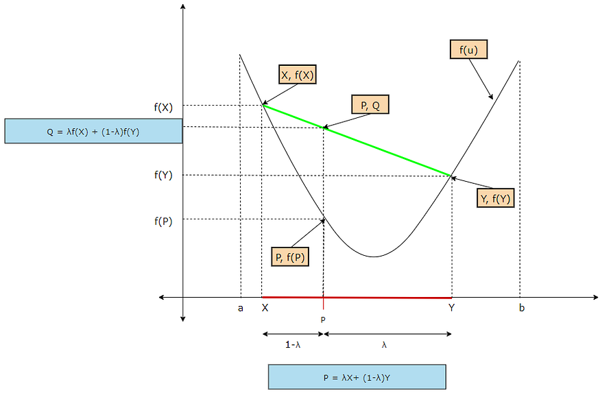
The first nine steps are the same as the proof of concavity. There is just a minor change in the algebraic proof. Here it goes…
1. Step — 1:
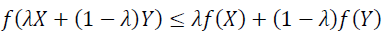
According to the definition of the concave function, the function f is concave if and only if for every pair of numbers X and Y with a≤ X ≤b and a≤ Y ≤b, we have…
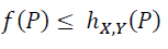
2. Step — 2:
The above condition must be true for every value 0≤ λ ≤1.
In conclusion, we can say that a function is convex when the above condition is met.
Now, we know that it is difficult to plot a graph of a function as the dimensionality of the function increases. So, we need to find another way to find out whether a function is convex or concave. Here come derivatives to our rescue!
A function f(x) is said to be a convex function if and only if f’’(x)>0 for all x. Here, f’’(x) refers to the second derivative of the function f(x). So, if we can prove that the second derivative of our loss function is >0, then we can claim it that the function is a convex function.
Visual proof of a convex function with an example
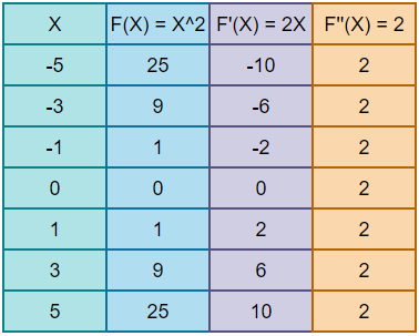
1. Step — 1:
We have our function f(X)=X². In the below image, we can see how the function f(X)=X² changes for different values of X. Notice that the value of f(X) is always positive.

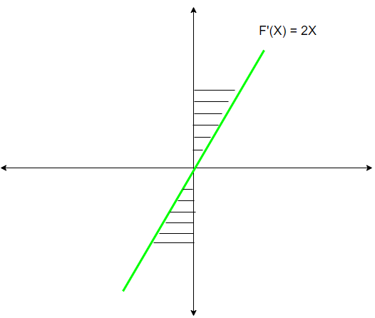
2. Step — 2:
Here we are plotting the derivative of F(X). The first derivative of a function is the rate of change of the function F(X). As we know that the rate of change of a function at any point is given by a tangential line drawn to that point. In the above image, we can see that when X<0, the rate of change is negative. When X=0, the rate of change is 0. When X>0, the rate of change is positive. Also, notice that for all values of X, as X increases, the rate of change of f(x) also increases. Refer to the following table to get a clear idea.
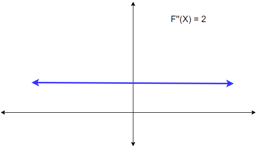
3. Step — 3:
Here we are plotting the graph of the second derivative of the function F(X). The 2nd derivative of a function is the rate of change of the 1st derivative of the function. In the above image we can see that for all values of X, the rate of change is always positive. (Tangent to any point is positive.)
Visual proof of a concave function with an example
Now, let’s take a concave function as an example to notice the differences between concave and convex functions.
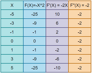
1. Step — 1:
We have our function f(X)=-X². In the below image, we can see how the function f(X)=-X² changes for different values of X. Notice that the value of f(X) is always negative.

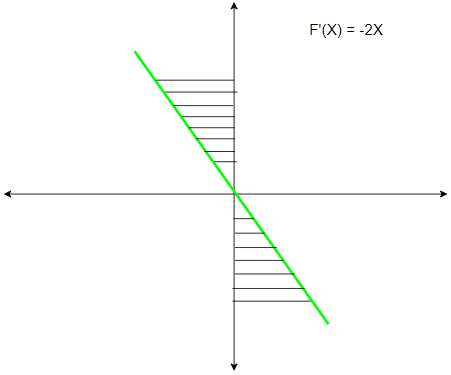
2. Step — 2:
Here we are plotting the derivative of F(X). The first derivative of a function is the rate of change of the function F(X). As we know that the rate of change of a function at any point is given by a tangential line drawn to that point. In the above image, we can see that when X<0, the rate of change is positive. When X=0, the rate of change is 0. When X>0, the rate of change is negative. Also, notice that for all values of X, as X increases, the rate of change of f(x) decreases.
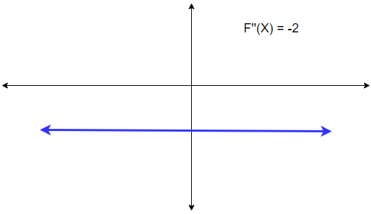
3. Step — 3:
Here we are plotting the graph of the second derivative of the function F(X). The 2nd derivative of a function is the rate of change of the 1st derivative of the function. In the above image we can see that for all values of X, the rate of change is always negative. (Tangent to any point is negative.)
Conclusion:
We can derive the following conclusions from it.
- If f’(X)>0, then f(X) is increasing.
- If f’(X)<0, then f(x) is decreasing.
- If f’’(X)>0, then f(X) is a convex function.
- If f”(X)<0, then f(X) is a concave function.
Based on the above proofs and derivations, we can confidently say that when the double derivative of a function is >0, then the function is convex and when the double derivative of a function is <0, then the function is concave. We are going to use these conclusions in the future.
In conclusion, the study of concave and convex functions is an essential component of mathematics and has far-reaching applications in numerous fields. Through this not-so-gentle introduction to concave and convex functions, we have explored the fundamental concepts, properties, and behavior of these functions. We have seen how the notions of concavity and convexity are related to optimization problems, and how they are used in real-world applications such as portfolio optimization, machine learning, and economics. Although the topic of concave and convex functions may seem daunting at first, it is an incredibly valuable and powerful tool for solving problems and making informed decisions. With a solid understanding of concave and convex functions, you can take your first step towards a more comprehensive understanding of mathematics, optimization, and data science.

Citation:
For attribution in academic contexts, please cite this work as:
Shukla, et al., “Unlocking the Power of Concave and Convex Functions in Machine Learning”, Towards AI, 2023
BibTex Citation:
@article{pratik_2023,
 title={Unlocking the Power of Concave and Convex Functions in Machine Learning},
 url={https://pub.towardsai.net/unlocking-the-power-of-concave-and-convex-functions-in-machine-learning-22b4adcdd690},
 journal={Towards AI},
 publisher={Towards AI Co.},
 author={Pratik, Shukla},
 editor={Binal, Dave},
 year={2023},
 month={Feb}
}
Resources and References:
Join thousands of data leaders on the AI newsletter. Join over 80,000 subscribers and keep up to date with the latest developments in AI. From research to projects and ideas. If you are building an AI startup, an AI-related product, or a service, we invite you to consider becoming a sponsor.
Published via Towards AI
Related posts


Popular posts

 for 2021")


Updates

Recent Posts


