Author(s): Manu Rastogi, Ph.D.

In recent times there has been a lot of interest in embedding deep learning models into hardware. Energy is of paramount importance when it comes to deep learning model deployment especially at the edge. There is a great blog post on why energy matters for AI@Edge by Pete Warden on “Why the future of Machine Learning is Tiny”. Energy optimizations for programs (or models) can only be done with a good understanding of the underlying computations. Over the last few years of working with deep learning folks — hardware architects, micro-kernel coders, model developers, platform programmers, and interviewees (especially interviewees) I have discovered that people understand LSTMs from a qualitative perspective but not well from a quantitative position. If you don’t understand something well you would not be able to optimize it. This lack of understanding has contributed to the LSTMs starting to fall out of favor. This tutorial tries to bridge that gap between the qualitative and quantitative by explaining the computations required by LSTMs through the equations. Also, this is a way for me to consolidate my understanding of LSTM from a computational perspective. Hopefully, it would also be useful to other people working with LSTMs in different capacities.

NOTE: The disclaimer here is that neither am I claiming to be an expert on LSTMs nor am I claiming to be completely correct in my understanding. Feel free to drop a comment if there is something that is not correct or confusing.

Why do we need RNNs?

Recurrent Neural Networks (RNNs) are required because we would like to design networks that can recognize (or operate) on sequences. Convolutional Neural Networks (CNNs) don’t care about the order of the images that they recognize. RNN, on the other hand, is used for sequences such as videos, handwriting recognition, etc. This is illustrated with a high-level cartoonish diagram below in Figure 1.

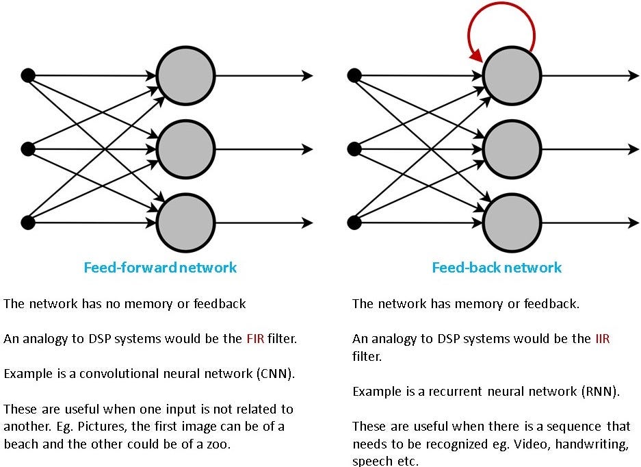
In a nutshell, we need RNNs if we are trying to recognize a sequence like a video, handwriting or speech. A cautionary note, we are still not talking about the LSTMs. We are still trying to understand the RNN. We will move to the LSTMs a bit later.

Cliff Note version

RNNs are required when we are trying to work with sequences.

RNN Training and Inference

In case you skipped the previous section we are first trying to understand the workings of a vanilla RNN. If you are trying to understand LSTMs I would encourage and urge you to read through this section.

In this section, we would understand the following:

1. Structure of an RNN.
2. Time unrolling

We will build on these concepts to understand the LSTM based networks better.

Structure of an RNN.

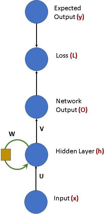
Shown in figure 2 is a simplistic RNN structure. The diagram is inspired by the deep learning book (specifically chapter 10 figure 10.3 on page 373).

A few things to note in the figure:

• I have stated the variables for each node in red color in the parenthesis. In the next diagram and the following section I will use the variables (in equations) so please take a few seconds and absorb these.
• The direction of the arrow from the expected output to the loss is not a typo.
• Variables U, V, W are the weight matrices of this network.
• The yellow blob in the feedback path (indicated by the green arrow) indicates the unit delay. If you are from DSP think of this as (z^-1)
• The feedback (indicated by the green arrow) is what makes this toy example qualify as an RNN.

Before we get into the equations. Let’s look at the diagram and understand what is happening.

1. At the beginning of the universe. Input ‘x(t=0)’gets multiplied with the matrix U resulting in x(t=0)*U .
2. The feedback from the last time step gets multiplied to the matrix W. Since this is the initial stage the feedback value is zero (to keep it simple). Hence the feedback value is h(t=-1)*W = 0. Thus the product is 0+x(t=0)*U = x(t=0)*U
3. Now, this gets multiplied with the matrix V resulting in x(t=0)*U*V.
4. For the next time step, this value will get stored in h(t) and will not be a non-zero.

Thus the above can also be summarized as the following equations:

In the above equations, we ignored the non-linearities and the biases. Adding those in the equations look like the following. Don’t worry if these look complicated.

Cliff Note version

RNNs have a feedback loop in their structure. This is what allows for them to work with sequences.

Time Unrolling

Time unrolling is an important concept to grasp for understanding RNNs and understanding LSTMs.

RNNs can also be represented as time unrolled version of themselves. It is another way of representing them nothing has changed in terms of the equations. Time unroll is just another representation and not a transformation. The reason we want to represent them this way is because it makes it easier to derive forward and backward pass equations. Time unrolling is illustrated in the figure below:

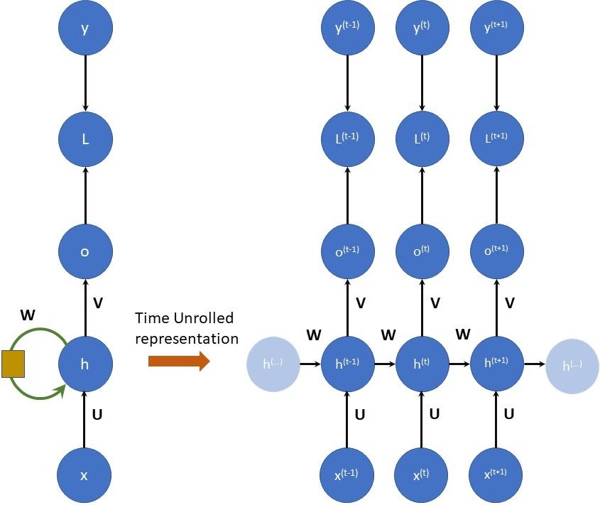
In the figure above the left side, the RNN structure is the same as we saw before. The right side is time-unrolled representation.

A few key takeaways from this figure:

1. The weight matrices U, V, W don’t change with time unroll. This means that once the RNN is trained the weight matrices are fixed during inference and not time-dependent. In other words, the same weight matrices (U, V, W) are used in every time step.
2. The lightly shaded h(..) on both sides indicate the time steps before h(t-1) and after h(t+1).
3. The above figure shows the forward (or the inference) pass of the RNN. At every time step, there is an input and a corresponding output.
4. In the forward pass, the “information” (or the memory) is passed onto the next stage through the variable h.

Cliff Note version

RNNs can be represented as time unrolled versions. This is just a representation and not a transformation. The weight matrices U, V, W are not time dependent in the forward pass.

Vanishing Gradient

RNNs suffer from the problem of preserving the context for long-range sequences. In other words, RNNs are unable to work with sequences that are very long (think long sentences or long speeches). The effect of a given input on the hidden layer (and thus the output) either decays exponentially (or blows and saturates) as a function of time (or sequence length). The vanishing gradient problem is illustrated in the figure below from Alex Graves’ thesis. The shades of the nodes indicate the sensitivity of the network nodes to the input at a given time. Darker the shade the greater is the sensitivity and vice-versa. As sown the sensitivity decays as we move from timestep =1 to timestep=7 very fast. The network forgets the first input.

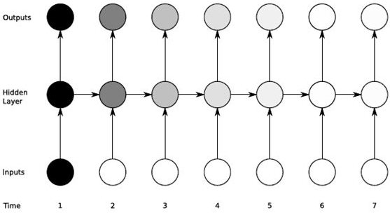
This is the key motivation for using LSTMs. The vanishing gradient problem has resulted in several attempts by researchers to propose solutions. The most effective of those is the LSTM or the long short-term memory proposed by Hochreiter in 1997.

Cliff Note version

Vanilla RNNs suffer from insenstivty to input for long seqences (sequence length approximately greater than 10 time steps). LSTMs proposed in 1997 remain the most popular solution for overcoming this short coming of the RNNs.

Long Short-Term Memory (LSTM)

LSTMs were proposed by Hochreiter in 1997 as a method of alleviating the pain points associated with the vanilla RNNs.

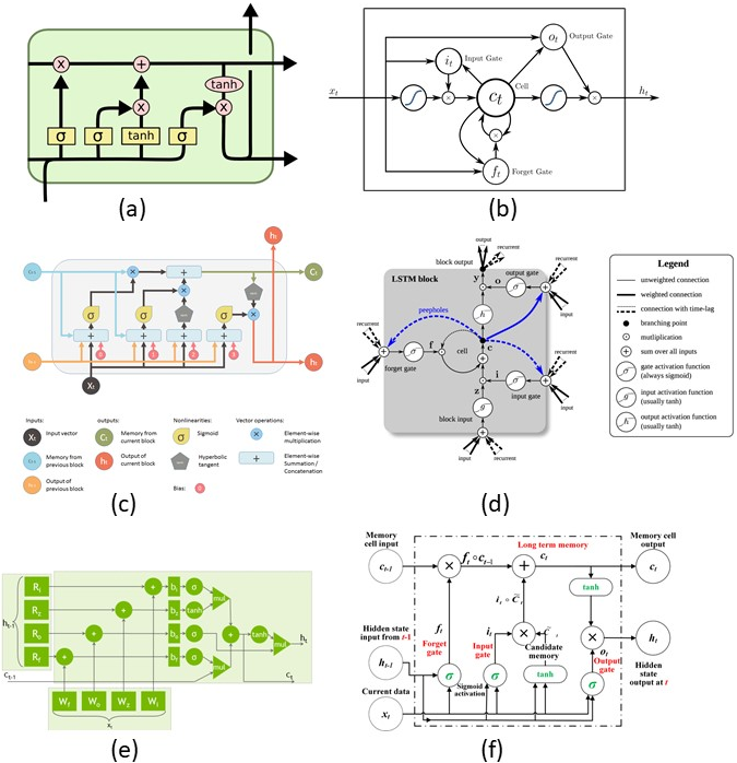
Several blogs and images describe LSTMs. As you can see there is a significant variation in how the LSTMs are described. In this post, I want to describe them through the equations. I find them easier to understand through equations. There are excellent blogs out there for understanding them intuitively I highly recommend checking them out:

(a) Christopher Olah’s blog.

(b) LSTM from Wikipedia

© Shi Yan’s blog on Medium

(d) LSTMs from the deep learning book

(e) Nvidia’s blog on accelerating LSTMs

LSTM equations

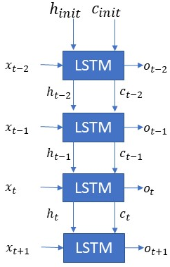
The figure below shows the input and outputs of an LSTM for a single timestep. This is one timestep input, output and the equations for a time unrolled representation. The LSTM has an input x(t) which can be the output of a CNN or the input sequence directly. h(t-1) and c(t-1) are the inputs from the previous timestep LSTM. o(t) is the output of the LSTM for this timestep. The LSTM also generates the c(t) and h(t) for the consumption of the next time step LSTM.

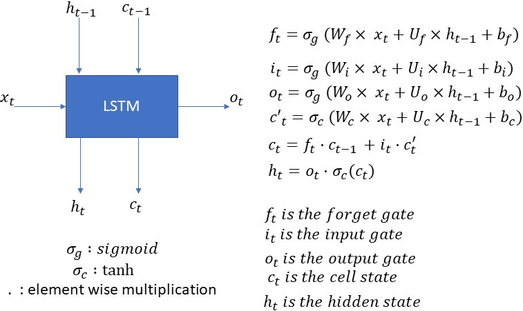
Note that the LSTM equations also generate f(t), i(t), c’(t) these are for internal consumption of the LSTM and are used for generating c(t) and h(t).

There are a few key points to note from the above:

1. The above equations are for only a one-time step. This means that these equations will have to be recomputed for the next time step. Thus if we have a sequence of 10 timesteps then the above equations will be computed 10 times for each timestep respectively.
2. The weight matrices (Wf, Wi, Wo, Wc, Uf, Ui, Uo, Uc) and biases (bf, bi, bo, bc) are not time-dependent. This means that these weight matrices don’t change from one time step to another. In other words to calculate the outputs of different timesteps same weight matrices are used.

The pseudo-code snippet below shows LSTM time computation for ten timesteps.

Code snippet illustrating the LSTM computation for 10 timesteps.

Cliff Note version

The weight matrices of an LSTM network do not change from one timestep to another. There are 6 equations that make up an LSTM. If an LSTM is learning a sequence of length ‘seq_len’. Then these six equations will be computed a total of ‘seq_len’. Essentially for everytime step the equations will be computed.

Understanding the LSTM dimensionalities

Armed with the understanding of the computations required for a single timestep of an LSTM we move to the next aspect — dimensionalities. In my experience, the LSTM dimensionalities are one of the key contributors to the confusion around LSTMs. Plus it’s one my favorite interview questions to ask 😉

Let take a look at the LSTM equations again in the figure below. As you already know these are the LSTM equations for a single timestep:

Let’s start with an easy one x(t). This is the input signal/feature vector/CNN output. I am assuming that x(t) comes from an embedding layer (think word2vec) and has an input dimensionality of [80×1]. This implies that Wf has a dimensionality of [Some_Value x 80].

Thus so far we have:

x(t) is [80 X 1] — input assumption

Wf is [Some_value X 80 ] — Matrix multiplication laws.

Let’s make another assumption the output dimensionality of the LSTM is [12×1]. Assume this is the number of output classes. Thus at every timestep, the LSTM generates an output o(t) of size [12 x 1].

Now since o(t) is [12 x 1] then h(t) has to be [12×1] because h(t) is calculated by doing an element by element multiplication (look at the last equation on how h(t) is calculated from o(t) and c(t)). Since o(t) is [12×1] then c(t) has to be [12×1]. If c(t) is [12×1] then f(t), c(t-1), i(t) and c’(t) have to be [12×1]. Why? Because both h(t) and c(t) are calculated by element wise multiplication.

Thus we have:

o(t) is [12 X 1] — output assumption

h(t) and c(t) are [12×1] — Because h(t) is calculated by element-wise multiplication of o(t) and tanh(c(t)) in the equations.

f(t), c(t-1), i(t) and c’(t) are [12×1] — Because c(t) is [12×1] and is estimated by element wise operations requiring the same size.

Since f(t) is of dimension [12×1] then the product of Wf and x(t) has to be [12×1]. We know that x(t) is [80×1] (because we assumed that) then Wf has to be [12×80]. Also looking at the equation for f(t) we realize that the bias term bf is [12×1].

Thus we have:

x(t) is [80 X 1] — input assumption

o(t) is [12 X 1] — output assumption

h(t) and c(t) are [12×1] — Because h(t) is calculated by element-wise multiplication of o(t) and tanh(c(t)) in the equations.

f(t), c(t-1), i(t) and c’(t) are [12×1] — Because c(t) is [12×1] and is estimated by element wise operations requiring the same size.

Wf is [12×80] — Because f(t) is [12×1] and x(t) is [80×1]

bf is [12×1] — Because all other terms are [12×1].

The above might seem a bit more complicated than it has to be. Take a moment and work through it yourself. Trust me it ain’t that confusing.

Now onto the confusing part 🙂 Just kidding!

In the calculation of f(t) the product of Uf and h(t-1) also has to be [12×1]. Now we know based on the previous discussion that h(t-1) is [12×1]. h(t) and h(t-1) will have the same dimensionality of [12×1]. Thus Uf will have a dimensionality of [12×12].

All Ws (Wf, Wi, Wo, Wc) will have the same dimension of [12×80] and all biases (bf, bi, bc, bo) will have the same dimension of [12×1] and all Us (Uf, Ui, Uo, Uc) will have the same dimension of [12×12].

Therefore:

x(t) is [80 X 1] — input assumption

o(t) is [12 X 1] — output assumption

Wf, Wi, Wc, Wo each have dimensions of [12×80]

Uf, Ui, Uc, Uo each have dimension of [12×12]

bf, bi, bc, bo each have dimensions of [12×1]

ht, ot, ct, ft, it each have a dimension of [12×1]

The total weight matrix size of the LSTM is

Weights_LSTM = 4*[12×80] + 4*[12×12] + 4*[12×1]

= 4*[Output_Dim x Input_Dim] + 4*[Output_Dim²] + 4*[Input_Dim]

= 4*[960] + 4*[144] + 4*[12] = 3840 + 576+48= 4,464

Lets verify paste the following code into your python setup

Notice the number of params for the LSTM is 4464. Which is what we got through our calculations too!

Before we move into the next section, I want to emphasize a key aspect. LSTMs have two things that define them: The input dimension and the output dimensionality (and the time unroll which I will get to in a bit). In literature (papers/blogs/code document) there is a lot of ambiguity in nomenclature. Some places it is called the number of Units, hidden dimension, output dimensionality, number of LSTM units, etc. I am no debating which is correct or which is wrong just that in my opinion these generally mean the same thing — the output dimensionality.

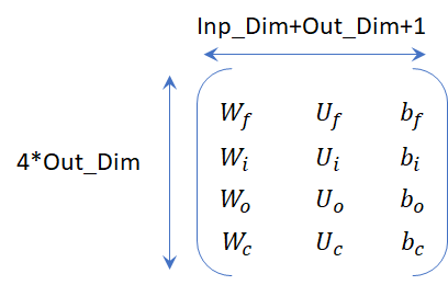
So far we have looked at the weight matrix size. The weight matrices are consolidated stored as a single matrix by most frameworks. The figure below illustrates this weight matrix and the corresponding dimensions.

NOTE: Depending on which framework you are using the weight matrices will be stored in a different order. As an example, Pytorch may save Wi before Wf or Caffe may store Wo first.

Cliff Note version

There are two parameters that define an LSTM for a timestep. The input dimension and the output dimension. The weight matrix size is of the size: 4*Input_Dim*(Output_Dim + Input_Dim + 1). There is a lot of ambiguity when it comes to LSTMs — number of units, hidden dimension and output dimensionality. Just remember that there are two parameters that define an LSTM — input dimensionality and the output dimensionality.

Time Unroll and Multiple Layers

In the figures below there are two separate LSTM networks. Both networks are shown to be unrolled for three timesteps. The first network in figure (A) is a single layer network whereas the network in figure (B) is a two-layer network.

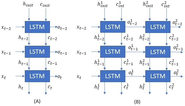
In the case of the first single-layer network, we initialize the h and c and each timestep an output is generated along with the h and c to be consumed by the next timestep. Note even though at the last timestep h(t) and c(t) is discarded I have shown them for the sake of completion. As we discussed before the weights (Ws, Us, and bs) are the same for the three timesteps.

The two-layer network has two LSTM layers. The output of the first layer will be the input of the second layer. They both have their weight matrices and respective hs, cs, and os. I indicate this through the use of the superscripts.

Example: Sentiment Analysis using LSTM

Let’s take a look at a very simple albeit realistic LSTM network to see how this would work. The task is simple we have to come up with a network that tells us whether or not a given sentence is negative or positive. To keep things simple, we will assume that the sentences are fixed length. If the actual sentence has fewer words than the expected length you pad zeros and if it has more words than the sequence length you truncate the sentence. In our case, we will restrict the sentence length to be 3 words. Why 3 words? just a number I like because it is easier for me to draw the diagrams :).

On a serious note, you would use plot the histogram of the number of words in a sentence in your dataset and choose a value depending on the shape of the histogram. Sentences that are largen than predetermined word count will be truncated and sentences that have fewer words will be padded with zero or a null word.

Anyways back to our example. We are sticking to three words. We will use an embedding layer which converts an English word into a numerical vector of size [80×1]. Why 80? because I like the number 80:) Anyways the network is shown below in the figure.

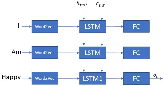
We will try and categorize a sentence — “I am happy”. At t=0 the first word “I” gets converted to a numerical vector of length [80×1] by the embedding layer. and passes through the LSTM followed by a fully connected layer. Then at time t=1, the second word goes through the network followed by the last word “happy” at t=2. We would like the network to wait for the entire sentence to let us know about the sentiment. We don’t want it to be overeager and tell us the sentiment at every word. This is why in the figure below the output from the LSTM is shown only at the last step. Keras calls this parameter as return_sequence. Setting this to False or True will determine whether or not the LSTM and subsequently the network generates an output at very timestep or for every word in our example. A key thing that I would like to underscore here is that just because you set the return sequences to false doesn’t mean that the LSTM equations are being modified. They are still calculating the h(t), c(t) for every timestep. Thus the amount of computation doesn’t reduce.

Here is an example from Keras for sentiment analysis on IMDB dataset:

https://github.com/keras-team/keras/blob/master/examples/imdb_lstm.py

Testing your knowledge!

Let’s try and consolidate what we have learned so far. In this section, I am listing a bunch of questions for some sample/toy networks. It helps me feel better if I can test if my understanding is correct hence this format in this section. Alternatively, you can also use these for interview preparation around LSTMs 🙂

Sample LSTM Network # 1

1. How many LSTM layers are there in this network? — The network has one layer. Don’t get confused with multiple LSTM boxes, they represent the different timesteps, there is only one layer.
2. As shown what is the sequence length or the number of timesteps? — The number of timesteps is 3. Look at the time indices.
3. If the input dimension i.e. x(t) is [18×1] and o(t) is [19×1] what are the dimensions of h(t), c(t)? — h(t) and c(t) will be of the dimension [19×1]

Sample LSTM Network # 2

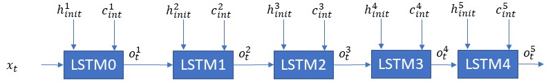
1. How many LSTM layers are there in this network? — The total number of LSTM layers is 5.
2. As shown what is the sequence length or the number of timesteps? — This network has a sequence length of 1.
3. If x(t) is [45×1] and h1(int) is [25×1] what are the dimensions of — c1(int) and o1(t) ? — c1(t) and o1(t) will have the same dimensions as h1(t) i.e [25×1]
4. If x(t) is [4×1], h1(int) is [5×1] and o2(t) is of the size [4×1]. What is the size of the weight matrices for LSTM0 and LSTM1? — The weight matrix of an LSTM is [4*output_dim*(input_dim+output_dim+1)]. The input dim for LSTM0 is [4×1], output_dim for LSTM0 is [5×1]. The input to LSTM1 is the output of LSTM0 thus the input dim of LSTM1 is same as the output_dim of LSTM0 i.e. [5×1]. The output dim of LSTM1 is [4×1]. Thus LSTM0 is [4*5*(5+4+1)]=200 and LSTM1 is [4*4*(5+4+1)] = 160.
5. If x(t) is [10×1], h1(int) is [7×1] what is the input dimension of LSTM1? — Look at the explanation above. We need to know the output dimensionality of LSTM0 before we can calculate this.
6. If x(t) is [6×1], h1(int) is [4×1], o2(t) is [3×1], o3(t) is [5×1], o4(t) is [9×1] and o5(t) is [10×1] what is total weight size of the network? — The weight matrix of an LSTM for a single timestep is given as [4*output_dim*(input_dim+output_dim+1)]. Work by estimating the input ouput dimensionalities of a single layer.

Sample LSTM Network # 3

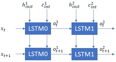
1. How many layers are in this network? — There are two layers
2. What is the sequence length as shown in this network? — Each layer is unrolled 2 times.
3. If x(t) is [80×1] and h1(int) is [10×1] what will be the dimensions of o(t), h1(t), c1(t), f(t), i(t). These are not shown in the figure, but you should be able to label this. — o(t), h1(t), c1(t), f1(t), i1(t) will have the same dimension as h1(t) i.e. [10×1]
4. If x(t+1) is [4×1], o1(t+1) is [5×1] and o2(t+1) is [6×1]. What are the size of the weight matrices for LSTM0 and LSTM1? — The weight matrix of an LSTM is given by 4*output_dim*(input_dim+output_dim+1). LSTM0 will be 4*5*(4+5+1) i.e. 200. LSTM2 will be 4*6*(5+5+1) = 264.
5. If x(t+1) is [4×1], o1(t+1) is [5×1] and o2(t+1) is [6×1]. What is the total number of multiply and accumulate operations? — I am leaving this one for the reader. If enough folks ask then I will answer 🙂

Sample LSTM Network # 4

1. How many layers are there? — There are 3 layers.
2. As shown how many timesteps is this network unrolled? — Each layer is unrolled 3 times.
3. How many equations will be executed in all for this network? — Each LSTM requires 6 equations (some texts consolidate to 5 equations). Then 6 equations/time step/LSTM. Therefore 6 equations * 3 LSTM Layers * 3 timesteps = 36 equations
4. If x(t) is [10×1] what other information would you need to estimate the weight matrix of LSTM1? What about LSTM2? — The weight matrix of an LSTM is given by 4*output_dim*(input_dim+out_dim+1). Thus for each LSTM, we need both input_dim and the output_dim. The output of LSTM is the input of LSTM1. We have the input dimension of [10×1] so we need the output dimension or o1(int) dimension and the output dimensions of LSTM1 i.e. o2(t). Similarly for the LSTM2, we need to know, o1(t) and o2(t).

Summary

The blogs and papers around LSTMs often talk about it at a qualitative level. In this article, I have tried to explain the LSTM operation from a computation perspective. Understanding LSTMs from a computational perspective is crucial, especially for machine learning accelerator designers.

References and Other links

DL Interview Preparation

Christopher Olah’s blog.

Shi Yan’s blog

LSTMs from the deep learning book

Nvidia’s blog on accelerating LSTMs

LSTMs on Machine Learning Mastery

Pete Warden’s blog on “Why the future of Machine Learning is Tiny”.

Bio: Manu Rastogi is a machine learning scientist at Hewlett Packard Labs in Palo Alto. Prior, Rastogi was part of the systems team at Qualcomm AI Research in San Diego. He earned his MS and Ph.D. at Computational Neuro Engineering Lab (CNEL) at the Electrical and Computer Engineering department at the University of Florida and his B.Tech from Dhirubhai Ambani Institute of Information and Communication Technology (DA-IICT) in Gandhinagar, Gujarat, India.

Tutorial on LSTMs: A Computational Perspective was originally published in Towards Data Science on Medium, where people are continuing the conversation by highlighting and responding to this story.

Published via Towards AI per author’s request.