


The Sigmoid Function: A Key Building Block in Neural Networks
Last Updated on July 25, 2023 by Editorial Team
Author(s): Towards AI Editorial Team
Originally published on Towards AI.
A complete guide to the sigmoid function
Author(s): Pratik Shukla
“The road to success and the road to failure are almost exactly the same.” — Colin Davis

Welcome! This tutorial is a deeper dive into one of the most prominent activation functions used in machine learning and deep learning. In this tutorial, you’ll learn about the sigmoid function and its derivative in detail, covering all its important aspects. We have included many graphs to help visualize the function and get a deeper understanding of how it works and how to use it. In the end, you’ll find some important code snippets related to the sigmoid function. You can run the code from this Google Collab file for interactive learning. Let’s get into it!
Table of Contents
- What is a sigmoid function?
- Properties of a sigmoid function
- Formulas of a sigmoid function
- Why do we need another variation of the sigmoid function?
- Understanding the range of a sigmoid function
- Need for a sigmoid function
- Some basic derivatives
- Theory about derivation
- Finding the derivative of a sigmoid function
- Another look at the sigmoid function
- Another perspective on the derivative of a sigmoid function
- Sigmoid and its derivative evaluated at x=0
- Code snippets
- References
What is a sigmoid function?
A sigmoid function is a mathematical function that has an “S”-shaped curve.


Properties of a sigmoid function:
- A sigmoid function can take any real number as an input. So, the domain of a sigmoid function is (-∞, ∞).
- The output of a sigmoid function is a probability value between 0 and 1. So, the range of a sigmoid function is (0, +1).
- The sigmoid function is given by this formula:

4. The value of a sigmoid function at x=0 is 0.5. So, we can say that σ(0) = 0.5.
5. The sigmoid function is monotonically increasing. This means that as the input value increases, the output value increases or remains constant, but it never decreases.
6. The function is continuous in the domain. This means that we can find the sigmoid value for any point on the curve.
7. The function is differentiable everywhere in its domain.
8. Sigmoid function has a non-negative derivative at each point. It shows that the graph of a sigmoid function never decreases.
9. The sigmoid function has only one inflection point at x=0. (An inflection point is a point where the curve changes the sign.)
10. The derivative of a sigmoid function is bell-shaped.

Formulas of a sigmoid function:
The sigmoid function can be defined by the following formulas.


Why do we need another variation of the sigmoid function?
The sigmoid function can be written in two equivalent forms as shown above. We need to have both equations because the first equation (Figure-6) takes care of the overflow for large positive values, and the second equation (Figure-7) takes care of the overflow for large negative values.
The above code snippets show the error we get if we don’t use the right formulas for extremely large and extremely small values.
Understanding the range of the sigmoid function:
The sigmoid function is given by…
Before moving on, let’s first have a look at the graph of e^-x and understand its range.

From the above graph we can derive the following conclusion:
- As the value of x moves towards negative infinity (-∞), the value of e^-x moves towards infinity (+∞).

2. As the value of x moves towards 0, the value of e^-x moves towards 1.

3. As the value of x moves towards positive infinity (+∞), the value of e^-x moves towards 0.

Now, let’s have a look at the graph of a sigmoid function.
From the above graph we can derive the following conclusions:
- As the value of x approaches negative infinity (-∞), the value of σ(x) approaches 0.
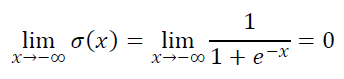
2. As the value of x approaches 0, the value of σ(x) approaches 0.5.
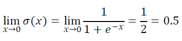
3. As the value of x approaches positive infinity (+∞), the value of σ(x) approaches 1.

The sigmoid function always gives the output in the range of (0,1).
Need for a sigmoid function:
Let’s take a very simple example to understand the need for a sigmoid function. Let’s say you’re a data scientist, and you are developing a model to predict whether a person will test positive for COVID-19 at a given point in time. Our model gives us a score based on various parameters. But, at this time, those parameters are not of our concern. Our model will output a score S ∈ (-∞, ∞). A higher score means that a particular person is likely to test positive and a lower score means that the particular person is not likely to test positive. Notice that at this point, we know that our model can give us a score ranging from (-∞, ∞). So, we don’t really know whether a particular score is higher or lower. At this point, we cannot say that a score of 1000 is high as the upper limit is +∞, in the same way, we cannot say that -1000 is low as the lower limit is -∞.
Suppose we took a survey and found out that the range of scores is (-100,100). Here we can say that 100 is a high score and -100 is a low score. So, we can say that a person with a score of 100 will test positive for COVID and a person with a score of -100 will not test positive. Now, here comes the tricky part! Suppose that we took the survey in a different region and the range of score is (-100000,100000). Here we can say that 100000 is a high score and -100000 is a low score. So, based on this we can say that a person with a score of 100000 will test positive for COVID and a person with a score of -100000 will not test positive for COVID. Now, if we combine both surveys then we will find out that the person in the first survey whom we said will test positive for COVID is not really positive. This is not the correct result. So, using just raw scores can be very problematic and inconclusive. We need to find a better way.
Somehow we need to make sure that the end results are always conclusive irrespective of the input domain. To do this, we can simply map the score to the probability values. Since we know that the probability values are always between 0 and 1, we don’t have to worry about the output range. This way we can make sure that we always have an output value between 0 and 1 irrespective of the input domain.
Now, in real life, when we are training a model, our score values are going to be some finite set of values. So, we need to make sure that even if our model is trained on a different domain, it returns conclusive values for the inputs outside of the domain. This is the only reason why we cannot use a straight line.

In the above graph, we can see that we have two data points at points x=-10 and x=10, respectively. In this graph, we have drawn a simple line to connect these data points. In the above graph, our domain is (-10,10) and the range is (0,1). By looking at the graph, we can say that it works perfectly. The maximum value is +10 and it is mapped to the probability of 1. The minimum value is -10 and it is mapped to the probability of 0. Any point between these data points can be mapped to their probability values by using the line. So, what is the problem here?
Issues:
- In the above graph, the values are in the range of (-10,10). Now, what happens if we have a point with values >10 or <-10? If we try to map it with the line then we will get some probability values >1 or <0, which doesn’t make any sense. In the below graph, we can see that if we use the previously trained model and if the new value is out of the domain then it gives the probability value greater than 1, which doesn’t make any sense. This is why we can’t use a straight line in this case.

2. The other issue is the rate of change in the line. We all know that the rate of change for any point on that line is always constant. But, in our case, we don’t want this characteristic. Suppose we found out that our domain is (-10,10). Here, -10 means that the person is not likely to test positive for COVID (P=0), and +10 means that the person is likely to test positive for COVID (P=1). Now, note that a score of 0 means that we don’t have much information about the person. So, there is a 50–50% chance of that person testing positive. Now, if we go from +9 to +10 or -9 to -10, it doesn’t make a big difference in a person tests positive or not. But, if we move from 0 to any direction, it makes a big difference. So, we need something other than a straight line that can take into account this sudden change. In short, here we need a high rate of change. On the other end, we know that in the extreme ends the severity of COVID doesn’t vary much. So, we need a low rate of change. That’s why we use an “S” shaped curve.
Some basic derivatives:
Let’s first have a brief look at some of the basic derivatives.
1. Derivative of e^x:

2. Derivative of e^-x:

Theory about derivation:
Let’s first derive the formula we are going to use to find the derivative of the sigmoid function, then put it to use to find the sigmoid function’s derivative.
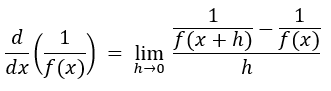
A. Step — 1:
The derivative of f(x) with respect to x is given as…

B. Step — 2:
This is the function for which we want to find the derivative.

C. Step — 3:
Now, we will use Figure-24 and plug its value into Figure-23.
D. Step — 4:
A simple cross multiplication.

E. Step — 5:
Taking out the negative sign (-) from the numerator.

F. Step — 6:
Dividing the formula into two parts.

G. Step — 7:
Giving individual limits to both parts.

H. Step — 8:
Definition of the derivative of f(x) with respect to x.

I. Step — 9:
As the value of h → 0, f(x+h) becomes f(x).

J. Step — 10:
Substitute the values of Step-8 and Step-9 into Step-7.

Finding the derivative of a sigmoid function:
Now, we will use the derived formula to find the derivative of a sigmoid function. The sigmoid function is given by…
A. Step — 1:

At this point, we need to find the derivative of f(x) and the square of f(x).
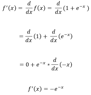
B. Step — 2:
Finding derivative of f(x).
C. Step — 3:
Finding the second part of the derivative.

D. Step — 4:
We will use this formula to plug in our values.

E. Step — 5:

This is the derivative of the sigmoid function. However, you’ll notice that we don’t generally see this format of the derivative of the sigmoid function. In fact, we can simplify the above formula to an easier and more efficient formula.
F. Step — 6:
Dividing the formula into parts.

G. Step — 7:

H. Step — 8:

I. Step — 9:

J. Step — 10:

So, this is the formula we generally use as a derivative of a sigmoid function. As we can see, it uses the previously calculated sigmoid values, so it is more efficient.
Another look at the sigmoid function:
Note that our sigmoid function σ(x) is rotationally symmetric with respect to the point (0,0.5). The sigmoid function and its reflection are symmetric about the vertical axis. The reflection of the sigmoid function about the vertical axis is given by σ(-x). We can also say that the sum of the sigmoid function σ(x) and its reflection about the vertical axis σ(-x) is 1 because the sigmoid function outputs the probability values and as we know that the sum of the probabilities in a probability distribution is always 1.

Mathematical Proof:

Another perspective on the derivation of a sigmoid function:
The sigmoid function for the positive values is given by…

The sigmoid function for the negative values is given by…

The derivative of the sigmoid function is given by…

Now, if we rearrange the terms, we can rewrite the derivative function in terms of σ(x) and σ(-x).

Since we know that the sum of the sigmoid function σ(x) and its reflection about the vertical axis σ(-x) is 1, we can say that…

We can also say that…

Sigmoid and its derivative evaluated at x=0:
In this section, we will evaluate the value of the sigmoid function and its derivative at x=0.
1. Value of a sigmoid function at x=0:


2. Value of the derivative of a sigmoid function at x=0:


Note that the value of a sigmoid function and its derivative evaluated at x=0 is always 0.5 and 0.25, respectively. It does not depend on the domain.
Code Snippets:
1. A graph of e^x:

The above graph shows that the value of e^x increases exponentially.
2. A graph of e^-x:
The above graph shows that the value of e^-x decreases exponentially.
3. A graph of e^x and e^-x:

The above graph shows a comparison of e^x and e^-x.
4. A simple graph of a sigmoid function:
The above graph shows how the output of a sigmoid function for a range of (-10,10).
5. A simple graph of a sigmoid function with its inflection point:
The above graph shows how the output of a sigmoid function for a range of (-10,10) with an inflection point at x=0.
6. A graph of a sigmoid function with larger domain values:

The above graph shows how the output of a sigmoid function for a range of (-100,100). Note that the values <-10 and >10 generate output nearly equal to 0 and 1 respectively. So, we can say that we can see many variations in the output of a sigmoid function only in the range of (-10,10).
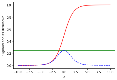
7. A graph of a sigmoid function and its derivation:

The above graph shows the plot of a sigmoid function and its derivative for the range of (-10,10).
8. A graph of a sigmoid function and its derivation with larger domain values:

The above graph shows the plot of a sigmoid function and its derivative for the range of (-100,100).
9. A graph of a sigmoid function and its derivation considering large positive and negative values:
The above graph shows the plot of a sigmoid function and its derivative for the range of (-10,10). Note that the above code works universally for extremely large and extremely small values of the input x.
10. A graph of a sigmoid function and its derivation considering large positive and negative values and a larger domain:

The above graph shows the plot of a sigmoid function and its derivative for the range of (-100,100). Note that the above code works universally for extremely large and extremely small values of the input x.
Conclusion:
That’s about it for this tutorial on the sigmoid function. We hope you enjoyed reading it and learned something new from it. You can experiment with the code snippets from this Google Collab file. Happy learning!

Citation:
For attribution in academic contexts, please cite this work as:
Shukla, et al., “The Sigmoid Function: A Key Building Block in Neural Networks”, Towards AI, 2023
BibTex Citation:
@article{pratik_2023,
 title={The Sigmoid Function: A Key Building Block in Neural Networks},
 url={https://pub.towardsai.net/the-sigmoid-function-a-key-building-block-in-neural-networks-c417a8748190},
 journal={Towards AI},
 publisher={Towards AI Co.},
 author={Pratik, Shukla},
 editor={Binal, Dave},
 year={2023},
 month={Feb}
}
References:
Join thousands of data leaders on the AI newsletter. Join over 80,000 subscribers and keep up to date with the latest developments in AI. From research to projects and ideas. If you are building an AI startup, an AI-related product, or a service, we invite you to consider becoming a sponsor.
Published via Towards AI
Related posts


Popular posts

 for 2021")


Updates

Recent Posts


