Support Vector Machine — Insights

Last Updated on June 19, 2020 by Editorial Team

Author(s): Gautam Kmr

Machine Learning

Support Vector Machine — Insights

I have talked about Linear regression and Classification on my prior articles. Before we take on to Support Vector Machine (aka SVM), let’s first understand what it does. The objective of the support vector machine algorithm is to find a hyperplane in N-dimensional space(N — the number of features) that distinctly classify the data points. It is highly preferred by many as it produces significant accuracy with less computation power. SVM can be used for both regression and classification tasks. But it is widely used in classification objectives.

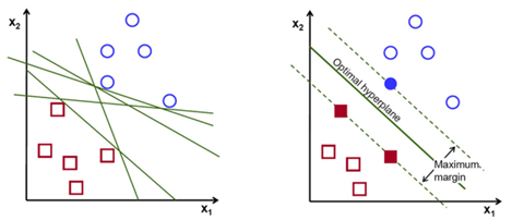
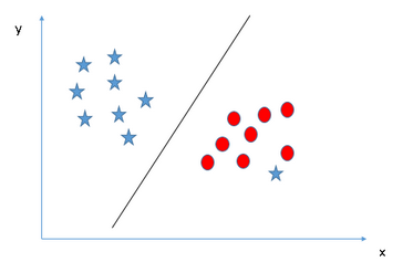
As seen in the first representation of the above figure, there could be multiple ways we can choose the hyperplane to separate the data points. However, our objective is to identify the plane with a maximum margin, i.e. the distance between the data points of both the classes should be maximum with the optimal hyperplane when compared to other hyperplanes.

How does it work?

Let’s understand the functionality of SVM using different scenarios:

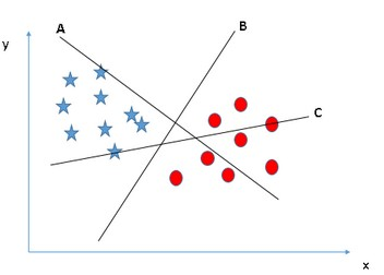
Scenario 1 — Here it’s pretty obvious from the below figure, that there are three hyperplanes to classify the data points however, the hyperplane B is defining the classification in a better way.

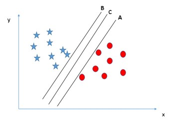
Scenario 2 — As we can see in the below figure, all three hyperplanes are defining the classification correctly. However, A & B has a very less margin for errors, i.e. they are very close to the data points. If there is any fluctuation in the data point values, they may fall into errors. The hyperplane C on the other hand has a significant margin for errors as it has the maximum distance from the data points of both the classes.

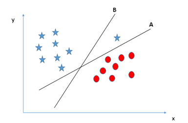
Scenario 3 — In the below scenario, we can see that there is one data point that can be considered an outlier. The hyperplane B has a better margin of errors however, SVM still chose the hyperplane A because it first identifies the hyperplane which classifies the data points better, and then it compares the margin of errors.

Scenario 4 — I mentioned in the previous scenario that the SVM first tries to identify the hyperplane which classifies the data better and then thinks about the margin of errors. However, in the below example we cannot classify the data points with a straight line. Hence, SVM ignores the outlier and selects the hyperplane which classifies the datapoint with a maximum margin of errors.

Scenario 5 — We have seen only linear classification with SVM so far however, in the below example it is not possible to have a linear hyperplane that can classify the data points.

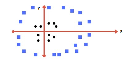
SVM solves this problem easily for us by adding another feature to the dataset.

Z = X2 + Y2 and plotting the datapoints on the X-Z axis instead of the X-Y axis.

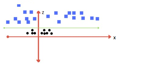
Now that we have a completely different picture of the dataset, we can easily identify the hyperplane on the X-Z axis.

There are a few things that we can notice in the above figure:

· The values on the Z-axis will always be positive as the squared sum of X and Y values

· The values of the circles (black) are closer to the origin of the X-axis in the actual dataset and the squares (blue) are comparatively far from the origin. Hence, the circles will always be closer to the origin and squares will be above that when seen on the Z-axis.

Data Preparation for SVM

This section lists some suggestions for how to best prepare your training data when learning an SVM model.

· Numerical Inputs: SVM assumes that the inputs are numeric. If we have categorical inputs, we may need to convert them to binary dummy variables (one variable for each category).

· Binary Classification: Basic SVM as described in this post is intended for binary (two-class) classification problems. Although, extensions have been developed for regression and multi-class classification.

SVM Tuning Parameters

In a real-world application, finding the perfect class for millions of training data sets takes a lot of time. There are some parameters that can be tuned while using this algorithm to achieve better accuracy.

Kernel

The learning of the hyperplane in linear SVM is done by transforming the problem using some linear algebra. This is where the kernel plays a role.

For linear kernel the equation for prediction for a new input using the dot product between the input (x) and each support vector (xi) is calculated as follows:

f(x) = B(0) + sum(ai * (x, xi))

This is an equation that involves calculating the inner products of a new input vector (x) with all support vectors in training data. The coefficients B0 and ai (for each input) must be estimated from the training data by the learning algorithm.

The polynomial kernel can be written as K(x,xi) = 1 + sum(x * xi)^d and exponential as K(x,xi) = exp(-gamma * sum((x — xi²)). [Source for this excerpt : http://machinelearningmastery.com/].

Regularization

The Regularization parameter (often termed as C parameter in python’s sklearn library) tells the SVM optimization how much you want to avoid misclassifying each training example.

For large values of C, the optimization will choose a smaller-margin hyperplane if that hyperplane does a better job of getting all the training points classified correctly. Conversely, a very small value of C will cause the optimizer to look for a larger margin separating hyperplane, even if that hyperplane misclassifies more points.

Gamma

The gamma parameter defines how far the influence of a single training example reaches, with low values meaning ‘far’ and high values meaning ‘close’. In other words, with low gamma, points far away from plausible separation lines are considered in the calculation for the separation line. Whereas high gamma means the points close to a plausible line are considered in the calculation.

Margin

And finally, the last but very important characteristic of the SVM classifier. SVM to core tries to achieve a good margin. A good margin is one where this separation is larger for both the classes. Images below give to the visual example of good and bad margins. A good margin allows the points to be in their respective classes without crossing to other classes.

Implementing SVM using Python

Python uses the SKLEARN library for the SVM algorithm.

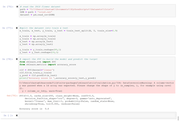
I have shown how does the SVM is applied to the IRIS flower dataset available on kaggle. SVM is a memory heavy algorithm and does take a long time on large datasets.

I will try to explain the fine-tuning of the SVM algorithm in my next article.

---

Support Vector Machine — Insights was originally published in Towards AI — Multidisciplinary Science Journal on Medium, where people are continuing the conversation by highlighting and responding to this story.

Published via Towards AI