Stock Price Change Forecasting with Time Series: SARIMAX

Last Updated on January 6, 2023 by Editorial Team

Author(s): Avishek Nag

Machine Learning, Statistics

High-level understanding of Time Series, stationarity, seasonality, forecasting, and modeling with SARIMAX

Time series modeling is the statistical study of sequential data (may be finite or infinite) dependent on time. Though we say time. But, time here may be a logical identifier. There may not be any physical time information in a time series data. In this article, we will discuss how to model a stock price change forecasting problem with time series and some of the concepts at a high level.

Problem Statement

We will take Dow Jones Index Dataset from UCI Machine Learning Repository. It contains stock price information over two quarters. Let’s explore the dataset first:

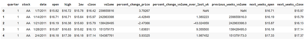
We can see only a few attributes. But there are other ones also. One of them is “percent_change_next_weeks_price”. This is our target. We need to forecast it for subsequent weeks given that we have current week data. The values of the ‘Date’ attribute indicate the presence of time-series information. Before jumping into the solution, we will discuss some concepts of Time Series at a high level for our understanding.

Definition of Time series

There are different techniques for modeling a time series. One of them is the Autoregressive Process (AR). There, a time series problem can be expressed as a recursive regression problem where dependent variables are values of the target variable itself at different time instances. Let’s say if Yt is our target variable there are a series of values Y1, Y2,… at different time instances, then,

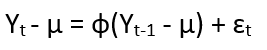
for all time instance t. Parameter µ is the mean of the process. We may interpret the term

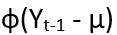
as representing “memory” or “feedback” of the past into the present value of the process. Parameter ф determines the amount of feedback and ɛt is information present at time t that can be added as extra. Definitely here by “process”, we mean an infinite or finite sequence of values of a variable at different time instances. If we expand the above recurrence relation, then we get:

It is called the AR(1) process. h is known as the Lag.

A Lag is a logical/abstract time unit. It could be hour, day, week, year etc. It makes the definition more generic.

Instead of the only a single previous value, if we consider p previous values, then it becomes AR(p) process and the same can be expressed as:

So, there are many feedback factors like ф1, ф2,..фp for AR(p) process. It is a weighted average of all past values.

There is another type of modeling known as MA(q) process or Moving Average process which considers only new information ɛ and can be expressed similarly as a weighted average:

Stationarity & Differencing

From all of the equations above, we can see that if ф or θ< 1 then the value of Yt converges to µ i.e., a fixed value. It means that if we take the average Y value from any two-interval, then it will always be close to µ, i.e., closeness will be statistically significant. This type of series is known as Stationary time series. On the other hand, ф > 1 gives explosive behavior and the series becomes Non-stationary.

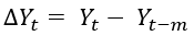
The basic assumption of time series modeling is stationary in nature. That’s why we have to bring down a non-stationary series to a stationary state by differencing. It is defined as:

Then, we can model ∆Yt again as time series. It helps to remove explosiveness as stated above. This differencing can be done several times as it is not guaranteed that just doing it one time will make the series stationary.

ARIMA(p,d,q) process

ARIMA is the join process modeling with AR(p), MA(q), and d times differencing. So, here Yt contains all the terms of AR(p) and MA(q). It says that, if an ARIMA(p,d,q) process is differentiated d times then it becomes stationary.

Seasonality & SARIMA

A time series can be affected by seasonal factors like a week, few months, quarters in a year, or a few years in a decade. Within those fixed time spans, different behaviors are observed in the target variable which differs from the rest. It needs to be modeled separately. In fact, seasonal components can be extracted out from the original series and modeled differently as said. It is defined as:

where m is the length of the season, i.e. degree of seasonality.

SARIMA is the process modeling where seasonality is mixed with ARIMA model.

SARIMA is defined by (p,d,q)(P, D, Q) where P, D, Q is the order of the seasonal components.

SARIMAX & ARIMAX

So far, we have discussed modeling the series with target variable Y only. We haven’t considered other attributes present in the dataset.

ARIMAX considers adding other feature variables also in the regression model.

Here X stands for exogenous. It is like a vanilla regression model where recursive target variables are there along with other features. With reference to our problem statement, we can design an ARIMAX model with target variable percent_change_next_weeks_price at different lags along with other features like volume, low, close, etc. But, other features are considered fixed over time and don’t have lag dependent values, unlike the target variable. The seasonal version of ARIMAX is known as SARIMAX.

Data Analysis

We will start by analyzing the data. We will also learn some other concepts of time series along with the way.

Let’s first plot AutoCorelation Function(ACF) and PartialAutoCorelation Function (PACF) using statsmodel library:

import statsmodels.graphics.tsaplots as tsa_plots

tsa_plots.plot_pacf(df['percent_change_next_weeks_price'])

And then ACF:

tsa_plots.plot_acf(df['percent_change_next_weeks_price'])

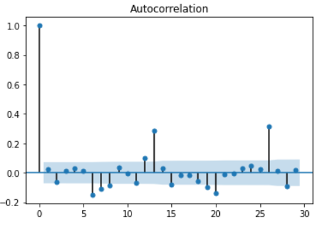
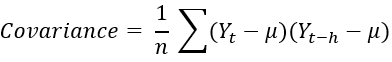
ACF gives us the correlation between Y values at different lags. Mathematically covariance for this can be defined as:

A cut-off in the ACF plot indicates that there is no sufficient relation between lagged values of Y. It is also an indicator of order q of the MA(q) process. From the ACF plot, we can see that ACF cuts off at zero only. So, q should be zero.

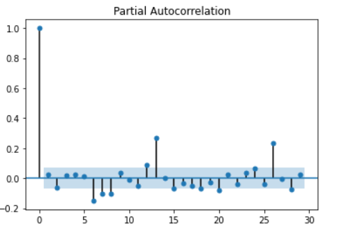
PACF is the partial correlation between Y values, i.e., the correlation between Yt and Yt+k conditional on Yt+1,..,Yt+k-1. Like ACF, a cut-off in PACF indicates the order p of the AR(p) process. In our use case, we can see that p is zero.

Decomposing components

We will now, how many components are there in the time series.

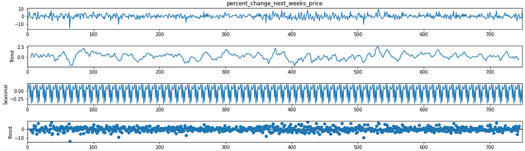
The first graph shows the actual plot, the second one shows the trend. We can see that there is no specific trend (upward/downward) of the percentage_change_next_weeks_price variable. But seasonal plot reveals the existence of seasonal components as it shows waves of ups & downs.

Stationarity check — ADF test

The characteristic equation of the AR(p) process is given by:

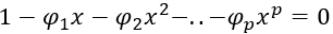
From our previous discussion, we can say that an AR(1) process is stationary if ф < 1 and for AR(p), it should be ф1 + ф2+..+фp <1. So the if the solution of the characteristic equation is of the form:

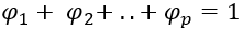
i.e, if it has unit-roots, then the time series is not stationary.

We can formally test this with Augmented Dicky-Fuller test like below:

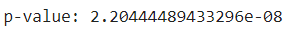
As the p-value is less than 0.05, so the series is stationary.

Building the model

We will start building the model.

Pre-processing

We will do some pre-processing like converting categorical variable stock to numerical, removing the ‘$’ prefix from price attributes, and fill all null values with zero.

We will also separate out the target & feature variables.

We will split the dataset into training & test.

TimeSeriesSplit incrementally splits the data in a cross-validation manner. We have to use the last X_train, X_test set.

Auto-modeling

We will use auto_arima from pmdarima library.

It tries out with different SARIMAX(p,d,q)(P,D,Q) models and chooses the best one. We used X_train as exogenous variables and seasonal start order m as 2(i.e., start from m for trying out different seasonal orders).

We got the output as below:

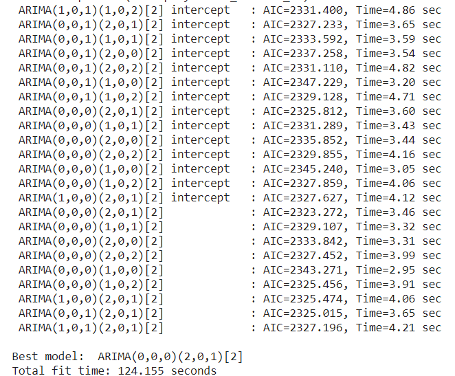
So, what we analyzed in the Data Analysis section came out true.

auto_arima checks stationarity, seasonality, trend everything.

The best model has p=0, q=0 and as the model is stationary, d=0. But, as we saw it has some seasonal components, its order is (2,0,1).

We will build the model with statsmodels and training dataset

Model details (clipped):

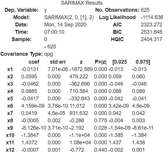
It shows all feature variable weights.

Forecasting

Before testing the model we need to discuss the difference between prediction & forecast. In a normal regression/classification problem, we use the term prediction very often. But, time series is a little different. Forecasting always considers lags into account. Here, to predict the value of Yt, we need value of Yt-1. And of course, Yt-1 will also be a forecasted value. So, it is a sequential & recursive process rather than random.

Mathematically, for an AR(2) process,

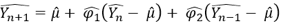
^Yn and ^Yn-1 are the previous forecasted values. This way the chain continues. In the case of ARIMAX, feature values are not dependent on time, so when we do a forecast, we feed previous Y values along with the same feature X values.

Now, its time to test the model:

from sklearn.metrics import mean_squared_error

mean_squared_error(result, Y_test)

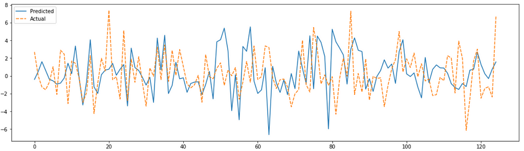
We will plot the actual vs predicted results.

We can also see the error distribution.

model.plot_diagnostics()
plt.tight_layout()
plt.show()

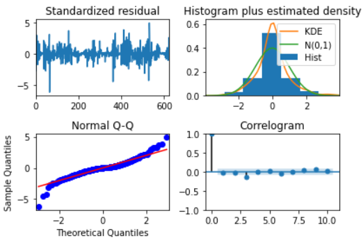
Errors are normally distributed with zero mean and constant variance which is a good sign.

Jupyter notebook can be found here:

avisheknag17/public_ml_models

Recently I authored a book on ML (https://twitter.com/bpbonline/status/1256146448346988546)

---

Stock Price Change Forecasting with Time Series: SARIMAX was originally published in Towards AI — Multidisciplinary Science Journal on Medium, where people are continuing the conversation by highlighting and responding to this story.

Published via Towards AI