Classic Methods for Identification of First Order Plus Dead Time (FOPDT) Systems

Last Updated on September 18, 2020 by Editorial Team

Author(s): Ricardo Guerra

Engineering

First Order systems are those whose input-output relationship is a first-order differential equation. These kinds of systems are very important, for example, The coffee machine as a mass heating system.

Therefore, the thing here is that sometimes we need to have the system model in hand to be possible to control them. But…

Sometimes it is difficult to obtain a system’s transfer function analytically. In many cases the system is closed, and one cannot identify its parts.

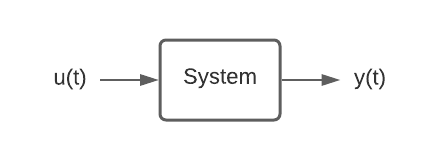
Is there a way we can fix things, and the way is by submitting the system to a step input, we can obtain from the system’s response to this entry important information that is difficult to access otherwise. In other words, the step response can lead us to find some attributes that make it possible to obtain the transfer function of the system.

Here we have a case to study: Imagine that for a temperature control system, assuming the length of the resistance wire R is negligible concerning the distance L that separates it from the thermometer and that the pipe diameter is small enough. We are talking about the problem illustrated in Figure 2.

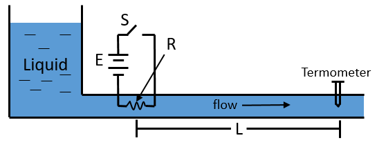
If the switch S is closed, the temperature of the liquid will rise immediately. However, until the thermometer as an output signal detects this, the heated liquid must reach the thermometer body, which will happen after a certain time that depends on the flow of the liquid. This time is what is called dead time. So, we are facing a First Order Plus Dead Time (FOPDT) system and for these systems, we have one equation associated with their dynamic response and its equation below.

Where:

• K = Process gain
• τ = Process time constant
• θ = Process dead time

Thus, the data from this example is available via the “data.mat” file containing the variables of time (t), step input u(t), and output y(t). The objective of the article is, using the data to implement the classic systems identification methods (using MatLab®) to obtain the first-order model of the system as:

• Ziegler-Nichols method;
• Smith’s method;
• Sundaresan’s method;
• Nishikawa’s method

All methods will be evaluated using the Mean Absolute Percent Error (MAPE), which is obtained through the equation below.

Where At is the current value and Pt is the predicted value and n is the number of samples.

Ok, so let’s start!

Ziegler-Nichols method

The method proposed by Ziegler, Nichols et al. (1942)[1], consists of applying a tangent line to the curve at an inflection point, to determine the system’s gain, time, and delay constants, as shown in Figure 3.

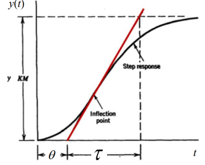
For the FOPDT, the response reaches 63% at instantet = θ + τ and the maximum tangent in response at t = θ intercepts y / KM in the line = θ + τ and so the step response has its state in permanent regime at t = 5τ (equilibrium time).

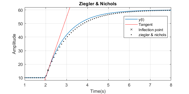
Applying the method in question, the dotted curve shown in Figure 4 is obtained. It is possible to notice that the curve was very close to the original, with a small difference. The MAPE for this problem was 0.65%.

The difficulty in applying this method is that it first becomes necessary to find the inflection point of the curve. The inflection points are defined where the curve changes direction and the derivative is equal to zero. In this case, this point was obtained by calculating the gradient to find the second derivative of the curve.

Then it becomes necessary to create a line tangent to the curve centered on the inflection point. After that, everything is easier because you just apply the method.

Smith’s method

Smith (1972)[2] proposed that the values of θ and τ be selected in such a way that the model and the real responses coincide in two points that present a high rate of variation. The intermediate values determined from the graph are the magnitude of the value applied in the input and the magnitude of the state of change in the output, being adopted two times, in which the first is when the output reaches 28%, and the second, 63% of the final value of the output, as illustrated in Figure 5.

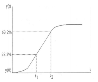
So, we can easily calculate t1 and t2 and then find:

Applying the method to the problem data, we obtain the dotted curve illustrated in Figure 6.

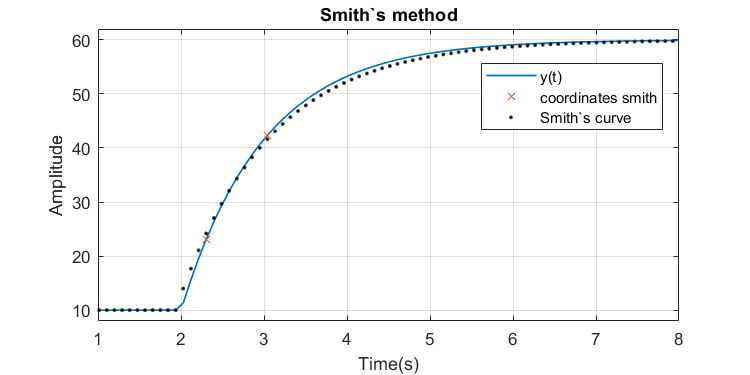
It is possible to notice that the curve was very close to the original, with a small difference. The MAPE for this problem was 0.513%, slightly better than the Ziegler-Nichols method.

Sundaresan and Krishnaswamy method

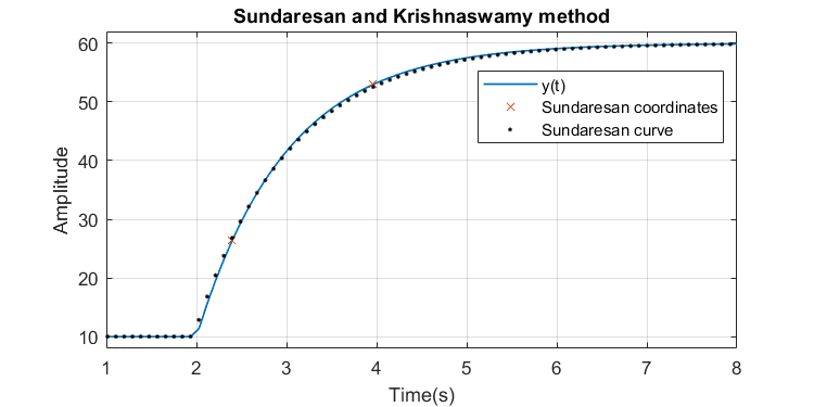
This method also avoids the use of the inflection point to estimate the time constant τ and transport delay θ. They proposed that two times, t1 and t2, be estimated from the one-step response curve, corresponding to 35.3% and 85.3% of the response, respectively.

The only difference concerning the Smiths method is the way the points are chosen and the way to find τ and θ which in this case is done through:

From the illustration in figure 7 it is possible to see that the predicted curve was almost identical to the original, reflecting in a MAPE of 0.2607%. In addition to a great result, this method is extremely simple and has a very low computational cost.

Nishikawa method

Nishikawa (2007)[3] created a method that consists of determining the values of the constants using the calculation of the curve areas as illustrated in Figure 8.

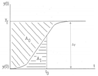
Where:

The model parameters are then obtained such that:

In this way, it is possible to obtain the curves illustrated in figure 9.

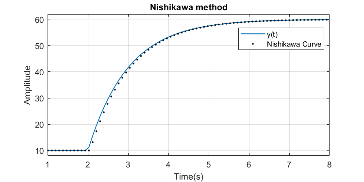
Once again, an excellent result is reflected through a MAP of 0.4195%, but with the cost of being a method with greater mathematical complexity and considerable computational cost, when compared to the others, since calculations of integrals are necessary to find the parameters of the system.

Conclusion

It was possible to study and apply the Ziegler / Nichols, Smith, Sundaresan, and Nishikawa methods, concluding that all obtained a considerably good result when computing a MAPE below 1% in all cases.

Some of the methods proved to be more complex, such as Ziegler and Nishikama, where in the first one it is necessary to find an inflection point and in the last one, perform area calculations, where, for this problem, they end up not bringing a result that justifies the increase in complexity. On the other hand, methods such as Smith and Sundaresan, besides being simple, achieved satisfactory results, with Sundaresan having the lowest MAPE.

An important observation for these methods is that, with the measures of response to real steps, the parameters K, τ and θ can vary considerably depending on the operating conditions of the process, that is, the magnitude of the step of entry and the direction of change. These variations can be attributed to the non-linearities of the process. Appendix A contains the MATLAB® code used to generate the results. If necessary, the code can also be found at my Github.

[1] ZIEGLER, J. G.; NICHOLS, N. B. et al. Optimum settings for automatic controllers.trans. ASME,v. 64, n. 11, 1942.

[2] SMITH, C. L. Digital computer process control. [S.l.]: Intext Educational Publishers, 1972.

[3] NISHIKAWA, H. A first-order system approach for diffusion equation. i: Second-order residual-distribution schemes. Journal of Computational Physics, Elsevier, v. 227, n. 1, p. 315–352,2007.

---

Classic Methods for Identification of First Order Plus Dead Time (FOPDT) Systems was originally published in Towards AI — Multidisciplinary Science Journal on Medium, where people are continuing the conversation by highlighting and responding to this story.

Published via Towards AI