


Preparing your Dataset for Modeling– Quickly and Easily
Last Updated on September 28, 2020 by Editorial Team
Author(s): Itamar Chinn
Data Science, Machine Learning
How to deal with categorical features and why SciKit makes things complicated but brilliant
This article is the second in a series that will walk you through a classic data science project. Hopefully, by now you have read Part 1 Exploratory Data Analysis (EDA) – ask what not how, if not, I recommend you read it before continuing.
Exploratory Data Analysis (EDA) — Don’t ask how, ask what
Overview
In this article, I will focus on the important elements of your dataset when preparing it for modeling, introduce some different methods to encode categorical features, and explain why an investment in the process at the beginning of your project will pay off in the end.
Why do we even have to prepare our dataset?
Once we have learned a bit about our dataset by doing EDA, we now want to prepare to model our data (the most exciting part of data science). Typically datasets are not given to us in a way that a model knows how to interpret so we need to clean the data, change it to a format that models can interpret, and apply any transformation that will allow us to produce the best possible model.
What can a model interpret? What does ‘clean’ even mean?
The answer to this question typically depends on the type of model you plan to use. For this project, I am going to prepare a tabular dataset to be modeled by a GBM (Gradient Boosting Machine — more on this in future episodes). I will also show which steps are important if I decide to use a different model later so that I can easily switch.
A model is a function and functions only like numbers. The preparation of a dataset is mainly changing your data (in any form — images, audio, labels for example) into a numeric format. I focus here on tabular datasets (dataframes) but the underlying principles hold for all types of data.
As data science becomes more accessible and used more, big modeling packages are becoming easier and easier to use, and so a lot of the process of preparing your dataset is no longer as manual as it used to be. For example, linear regression models require that the data is normalized otherwise it will just give preference to features with the largest inputs. Once this meant you had to scale the data manually, but now — as it is in SciKit-Learn — most packages leave this to a simple keyword argument in the fit method. Another example is in GBM models, often you don’t even need to change labels to numeric values, you just need to note which features are categorical (see the documentation for LightGBM here or some discussion on how good LightGBM does categorical encoding on Kaggle).
But as we will discover, if you understand why a certain feature needs to be encoded in a certain way, then your model will be much more accurate.
SciKit-Learn Encoder’s Fit and Transform

I want to make one point before getting into it, if you take away one thing from this article I hope it is this:
Always use fit and transform — sorry pd.get_dummies
Even if you think you know exactly how a project will turn out, you should always build your code and process in a way that will allow for maximum flexibility in the future.
As you will learn in this article, there are many methods of encoding your categorical features, but most of them don’t take into account the many different ways you might use your dataset further down the line.
Example of the importance of using fit and transform
In SciKit-Learn almost every module has a .fit and .transform method. This structure for processing your dataset came about for many reasons, but mainly to build a data pipeline that is robust regardless of changes in the input. You should never assume that the data will come exactly as it has in the dataset you’re currently working on.
What does that mean? Let’s say I am working on our diabetes readmission rate model again, the dataset has 50 input features (including several ones we will eliminate in a second). Let’s say I go through the entire process of modeling the data and my model’s accuracy is not good enough, so I manage to get access to another dataset, but this dataset has only 47 of the features, if I “hardcode” (create a process that only knows how to deal with 50 input features) the entire process then my code will crash. Usually the process of creating a set of actions on data that ends in modeling and actions is called building a pipeline. We want our pipeline to deal with changing data as best it can.
The benefit of using SciKit’s fit and transform methods is that you can build a pipeline for your data that is robust across changing inputs. “Fit” basically means that SciKit checks your data and creates a platform for the change, and then “transform” applies that platform to the dataset. So if suddenly the new data has less categories that are encoded as one-hot vectors (scroll down for more on this), the “transform” step will know how to take this into account. A pipeline that has a “hardcoded” stage will just crash if the input is different. Another possible and very typical change in input data is even just the order of the columns, if we have ‘hardcoded’ to encode column 3 in one-hot vector encoding, if the columns are rearranged we could ruin the entire dataset.
Inverse-ing Data to its Original Form
The other major benefit of using ‘fit’ and ‘transform’ is that we may want to analyze our dataset beyond just modeling it. Let’s say we encode all of our categorical variables and model the data. Then we use SHAP (more on SHAP in future articles) to understand our model, but want to also visualize what we learn, we want to see the decoded data (functions like numbers, but humans like labels). Many of the encoding modules in SciKit-Learn have an inverse method that decodes the data back into its original form.
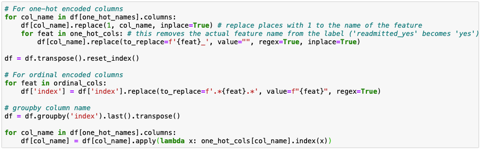
Let’s look at an example of decoding a dataset manually vs. using SciKit inverse. Here’s an example of how horrible it can be to do manually:
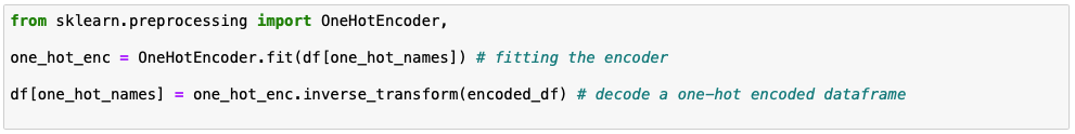
Or using SciKit inverse_transform:
Lets get to it then

Steps
The steps preparing your dataset for modeling are usually as follows:
- Remove difficult to fix or useless features
- Double check numeric features
- Identify relationships of labels in categorical features (binary, ordinal, or nominal)
- Reduce dimensions of high-cardinality features
- Encode
1 — Remove difficult to fix or useless features
There are features that won’t help us in modeling the data — this includes any features that we won’t have at the time of prediction (for example ‘Reason for Readmission’ because this is based on ‘Readmission’ and that is what we are trying to predict) or any feature that doesn’t help add new information to the model.
Let’s take a look at some of these in our diabetes dataset.
Unique Values
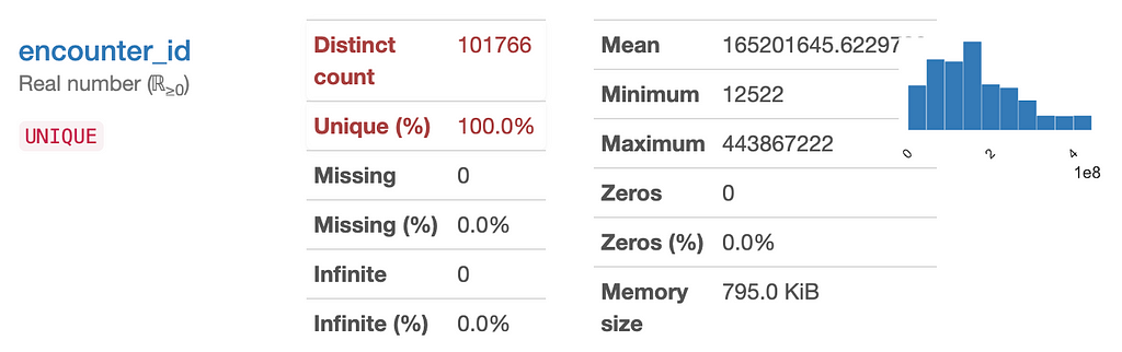
One of the clearest examples is “encounter_id” which is a unique ID that was given to every patient. We can get rid of this, since an ID number does not add information about a patient that can help predict their readmittance.
Another one that needs to be checked is ‘patient_nbr’ because we expect that each patient has a unique one, so this might indicate that we have duplicate rows since only 70% of samples have unique ‘patient_nbr’s. After removing any duplicate rows, we can get rid of this feature too since it won’t effect the prediction of the model.
Constant
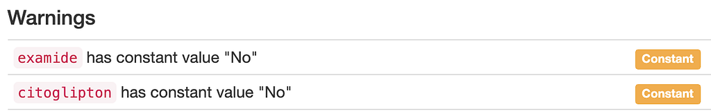
If all the samples in the dataset have the same input for a specific feature, then this feature can’t help us predict the target. In the Pandas Profiling ‘Warnings’ tab, we can easily identify these features, such as ‘Examide’ and ‘Citoglipton’ where all samples have the input ‘No’. We can therefore get rid of this feature too.
Many Missing Values
Another potential feature to remove is one with many missing values. If we are missing the values for many of the samples, it may be create false predictors for our model. Let’s say every patient that was readmitted was asked how many children they had, and so only patients that were readmitted had this data, then it would be easy for the model to learn that if there is a value for ‘Number of Children’ then there is a high probability of readmittance. In our dataset, for example, we are missing the ‘weight’ of most patients:

I would get rid of this feature as well since it will be hard to justify any value we give for weights since 99% of the samples are missing data.
I urge you to read more into missing values before making any final decisions whether or not to remove a feature, I have expanded on the topic in part in my first article Part 1 — EDA, but many sources go into the complexity of dealing with missing values in depth).
Leakage
This is sometimes hard to identify and might come up only after the modeling stage of the project, but a great example of a feature that might need to be removed is ‘Admission_Type_ID’ . There are 8 unique entries for this feature, and perhaps one of them is an ID for those who are readmitted— this is called model leakage because when we’re trying to predict if the patient will be readmitted then if we know they have already been readmitted, we have the answer. The model would likely identify this as the strongest predictor of readmission if we did not remove it, but also the model would be useless for unseen data.
2 — Double check numeric features
For numeric features, it is easiest if we use the same data type for all. I recommend always using numpy floats. The diabetes dataset gives another great example of why we need to double-check this. Let’s look at ‘Age’:
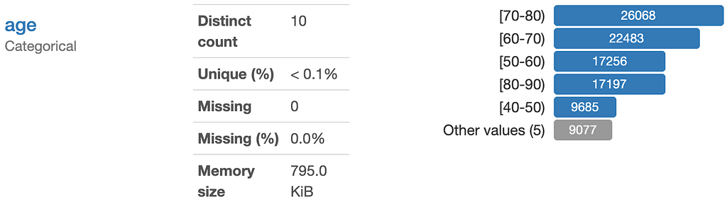
It looks like a classic numeric feature, but if we check the datatype we note it is actually a string.
Simply go through the features one by one and change all the numeric ones to numpy floats (df.astype(np.float64, inplace=True) should work).
3 — Identify relationships of labels in categorical features
Welcome to the hard (but fun!) part. Categorical features are the features that are given to us as a label, but that we want to turn into a number for the model (remember functions like numbers, humans like labels). There are a few different labels that we might come across though. I will discuss the different types of features, explain how I recommend encoding them, and then give an example from our dataset on how to do this.
What does encoding them mean?
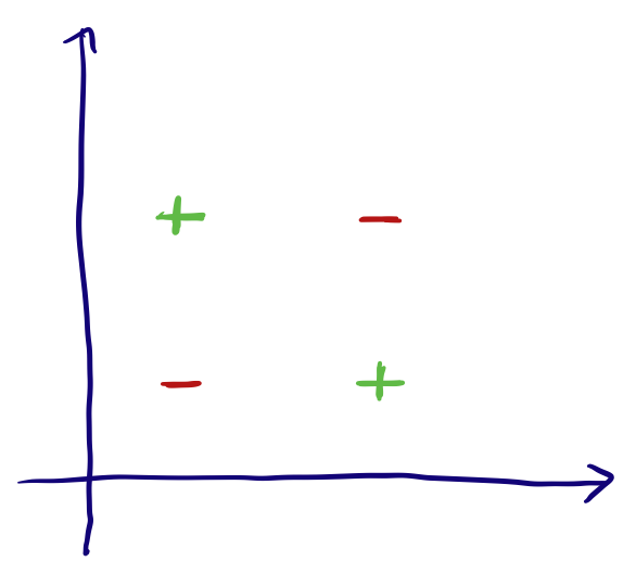
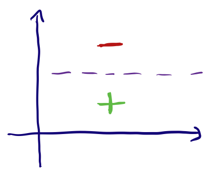
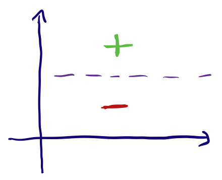
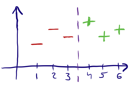
In the end, we will be modeling our data using mathematical functions. An easy way to understand the encoding of categorical data is as feature transformations that allow us to make our data separable after certain dimensions (although this isn’t necessarily what we are doing and depends on the model used).

Binary
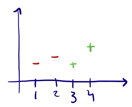
Binary features are ones where the inputs are one of two options (Yes/No, High/Low, Soft/Hard, etc). We can deal with them pretty simply by them as 0 or 1. Again we can easily see why this is acceptable since it shouldn’t affect the modeling regardless of how we label each:
Ordinal
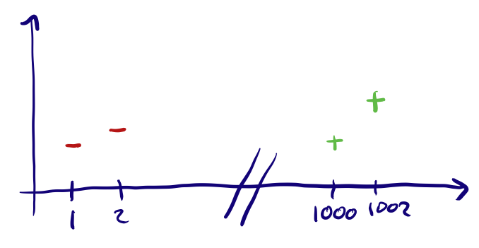
Ordinal features are ones where the input range can be measured on a scale, or where the order of the input matters. Some examples of this are: Very High, High, Medium, Low, Very Low (5 being Very High to 0 being Very Low) which is not the same as a scale Low, Very High, Very Low, High, Medium (5 being Low and 0 being Medium). These are a bit trickier to encode, the way to do this is by assigning a value to each label and simply encoding according to this mapping. This might be hard if the scale is not exactly as simple, let’s say we had a feature “Rockiness” with inputs ‘No Rocks’, ‘A lot of rocks’ and ‘Millions of rocks’. A mapping of No Rocks’ : 0, ‘A lot of rocks’ : 1 and ‘Millions of rocks’ : 2, might be incorrect and a better mapping might be No Rocks’ : 0, ‘A lot of rocks’ : 100 and ‘Millions of rocks’ : 1000000 (this also depends on the model you end up using).
Another option for data like this is using a ‘thermometer’ encoding as explained very well in this article.
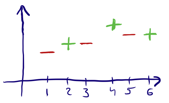
Nominal
Nominal features are ones where the inputs are simply labels that have no specific order or value to them. Typically we encode these as One-Hot Vectors, unless there are many different labels (high-cardinality features), in which case there are a few different methods to reduce the number of labels and then encode them.
A Note of Caution
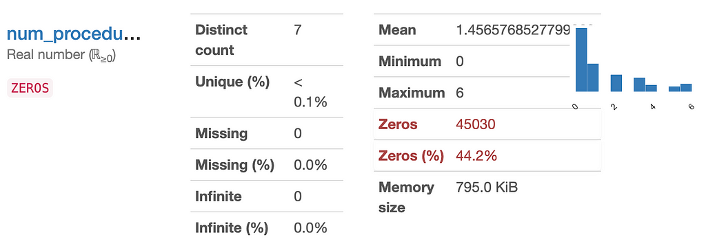
Be careful when doing this though, because some features might appear to be disposable but in reality be very indicative of your target! Take “Number of Procedures” for example, here most patients had 0 procedures done, but we can imagine that this might be a good predictor.
4 — Reduce dimensions of high-cardinality features
A hot source of controversy in the machine learning community, there is no right answer to how to reduce the dimensions of features with high-cardinality. What are features with high-cardinality? Let’s say we have a feature with 100 different labels (maybe we have a feature of ‘Medicine Brands’ and there are over 100 brands of medicines), then we would have to encode this feature using one-hot vectors, but this would create 100 new features which will highly increase the dimension of our model which we typically want to avoid.
I will explain some of the commonly used and quick methods for 99% of applications but do note that there are some very sophisticated methods to handle this that I will not go into.
Grouping — One easy solution, is to group labels. For example, most medications have several different brands with identical active ingredients or use-cases. We can mark all the brands with the same use-case or active ingredient by this name, and then use one-hot encoding by this grouping.
Counting or Sums — For non-linear algorithms in particular, you can replace the label with the number of times it appears in the dataset (sometimes known as count encoding, you can read about this on Kaggle here)
Cutoffs — Often a few of the labels in our high-cardinality feature appear most of the time, and others appear much less. In this case, we can often define a cutoff, such as 10%, and any label that appears less than 10% of the time we can simply give the label “Other”. If after the modeling step we discover that ‘Other’ is a high indicator of our target, then we might want to return to this step and think of another method.
Encoding features with high-cardinality is often very dependent on the model used and the dataset, and so I recommend that when doing this you explore further what methods have been used in a similar context to the project you are working on. Some alternative methods (more complex and often not as effective as the more simple methods) and links are: Feature Hashing , Target Encoding (which has many similar siblings such as LeaveOneOut Encoding and M-Estimate Encoding), Entity Embeddings, and many many more.
5 — Encode
Now you’re ready! You’ve removed the difficult to fix or useless features, double-check numeric features, identified the relationships of labels in categorical features (binary, ordinal, or nominal), and noted them, and finally reduced the dimensions of high-cardinality features and you’re ready to encode them.
As I explain in my note on using SciKit’s fit and transform, this is the stage to go to SciKit’s documentation (with emphasis on the ‘preprocessing’ module) and find the relevant functions to encode the different features. Here are some that will help you with the types of features described in this article:
- MinMaxScaler (to standardize data for linear models for example)
- OneHotEncoder (can be used for binary as well, I recommend this article for a step-by-step walkthrough)
- OrdinalEncoder
Conclusion
Preprocessing your dataset is something you are probably going to spend a lot of your time doing, and so it is essential to understand why it is important, and also what are best practices that will make your life easier later on in your project.
In this article, I don’t dive too deep into exactly what code to run (as it is rather simple if you read the SciKit documentation), but rather explain what is happening to the data when we encode it, and why it is so critical to get it right.
You’re now done with the most labor-intensive steps of your project! Give yourself a pat on the back, and now it’s time to really put our thinking caps on before we jump into the real data-science nitty-gritty — feature engineering and modeling — coming soon!
Lastly, I would like to point any readers to a really great resource to take your first steps in machine learning: MIT’s Introduction to Machine Learning course, which can be taken for free online here. I know how hard it is to find good courses (and especially for free) online in the sea of resources out there — so I can promise you this is a good one.
Stay tuned for the next steps in a classic data science project
Part 1 Exploratory Data Analysis (EDA) — Don’t ask how, ask what.
Part 2 Preparing your Dataset for Modelling — Quickly and Easily
Part 3 Feature Engineering — 10X your model’s abilities
Part 4 What is a GBM and how do I tune it?
Part 5 GBM Explainability — What can I actually use SHAP for?
(Hopefully) Part 6 How to actually get a dataset and a sample project
Preparing your Dataset for Modeling– Quickly and Easily was originally published in Towards AI — Multidisciplinary Science Journal on Medium, where people are continuing the conversation by highlighting and responding to this story.
Published via Towards AI
Related posts


Popular posts

 for 2021")


Updates

Recent Posts


