Physics Informed Neural Networks — Case Study of Quantitative Structure-Property Relationships

Author(s): Kamil Oster

Originally published on Towards AI.

Physics Informed Neural Networks — Case Study of Quantitative Structure-Property Relationships

Hi!

I came across the term Physics-Informed Neural Networks (PINNs). Please follow me on this journey to explore one of the case studies I have decided to investigate further.

First things first — what are PINNs?

Neural Networks are thought to be black-box models (data come in and come out without much information as to what happens inside that box, a.k.a. model). With this in mind, while inference is what we want out of this box, it has certain limitations. For example, considering simple multilayer perceptron (MLP) neural networks, there is a need for more information about how good the predictions are (what is the confidence in the predictions?) or how these predictions were achieved (any understanding of what is happening inside that box). Of course, there are ways to reach a level of understanding for all these [1a][1b][1c]. However, they are never 100% confident and come with their own limitations. There are multiple solutions to these problems, and one of them can provided by PINNs.

In layman’s terms, neural networks take a set of inputs, perform computation on a collection of weights and biases (grouped into so-called layers), filter against activation functions, and finally reach the set of outputs (these operations are referred to as forward propagation). The predicted output is compared against the ground truth (actual output values) with loss function (e.g. MSE, MAE, Huber, etc.). The loss function is essential information to an optimiser (e.g. Adam, LBFGS, etc.), which will update weights and biases of each hidden layer (these operations are referred to as backward feed or backpropagation). The process continues until a satisfactory level of performance is reached.

There is a level of assumption that the neural network will be capable of learning patterns that we would normally observe from a domain knowledge point of view, which they will learn through meticulous training. What if we can guide the training to learn the right patterns that we would expect? This is where PINNs come into play. PINNs are highly tailored to the problem, i.e., multiple strategies can convert your MLP problem into a PINN problem. In a PINN, the neural network is augmented with additional equations that represent the underlying physics of the problem. These equations act as constraints during training, guiding the network to learn the correct patterns. You will find multiple tutorials and readings covering complex applications of PDEs, etc [2a][2b][2c]. Do not be discouraged by that — PINNs do not have to be that difficult to understand (particularly for people with less mathematical or science background) — PINNs is an umbrella name for any NN-based models that contain theory-based functions to guide the model training into a more theory-based level.

I have applied one of the approaches in this case study, so please follow this article for more information. Libraries are available to train PINN models (links at the bottom) [3a][3b][3c]. However, writing your own code brings a lot of flexibility as to how you apply PINNs.

Case Study — Quantitative Structure-Property Relationship for the Prediction of Density as a Function of Temperature and Pressure

Quantitative Structure-Property Relationship (QSPR) is a term used in computational chemistry for correlations and predictions of chemical and physical properties of molecules based on their molecular structure (also called molecular descriptors). Most simply, molecules are like Lego blocks — they are built of blocks that reflect on their structure. For example, green — carbon, blue — oxygen, red — hydrogen (colours are arbitrary), etc. By choosing the right colour, size, and shape of the block, one could build a molecule. There are multiple ways to decompose molecules into these primary pieces (these pieces are often big functional pieces of a molecule). This allows us to ‘build’ molecules that have specific properties that we want, for example, chemical (such as efficacy for certain chemical reactions), physical (such as viscosity, density, etc.), biological (such as affinity to react with proteins), and much more! It is used almost everywhere — it is rare that we go to the lab and create molecules to investigate their properties. We design the molecules on a computational level to have certain properties and then validate them through an experimental route. While it might be completely new to the reader, let me give you an example to which you can relate. Let’s go back to April 2020, when covid-19 hit. How do you think they could have developed a vaccine so quickly? A-ha! QSPR (amongst many other methods!) were the knight in shining armour. Pharmaceutical concerns already had a lot of expertise in designing pharmaceuticals to target specific biological processes, such as those responsible for fighting COVID-19.

In this case study, we will focus on a simpler QSPR. More specifically, we will explore how to predict the density of so-called ionic liquids (ILs) under elevated temperature and pressure. The process involves training a PINN model using a dataset of ILs with known density values at various temperature and pressure conditions. The model will then be used to predict the density of new ILs under different temperature and pressure conditions. ILs are liquids composed solely of ions (i.e. cations and anions). Therefore, they have unique properties — such as low volatility, high boiling point, and high thermal stability. Because of their structure, they are easy to tailor the cation and/or anion to achieve certain properties. However, they are not the easiest to synthesise (they are prone to absorb water, so any measurements can be skewed easily) and are very expensive. If the reader is interested to know more about ILs, please refer to the references at the end of the article [4]. QSPR is a true hero in designing new ILs to reduce the cost and synthesis complexities. I have used a dataset published by Kamil Paduszynski (link below). You will need to pay to download the article. However, supporting information which contains the data is free of charge (link at the bottom). [5]

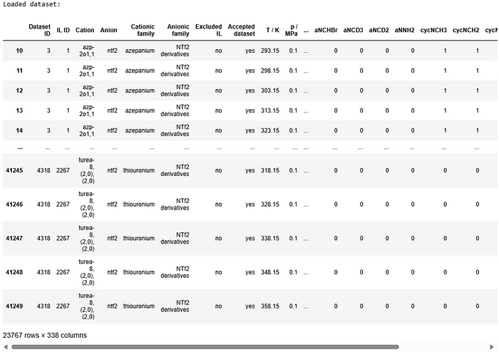
Dataset

All codes and relevant data are available in a Git repository referenced at the end of the article [6]: kamil2oster/QSPR_PINNs (github.com).

The original data published by the author were extracted. 41,250 data points were collected. The authors have reviewed data quality and provided information on which dataset has been used for further research. After narrowing down the accepted datasets, 23,989 data points were extracted. In total, 1,287 cation-anion pairs were available. For the simplicity of this article, only ILs with a cation:anion ratio of 1:1 were taken (resulting in a dataset consisting of 23,767 data points). I will not discuss how the data were extracted and cleaned initially. The notebook is available on my GitHub (link at the bottom of the page) [7].

The inputs consisted of 320 ILs structure-related descriptors, molar mass (M in g/mol), temperature (T in K), and pressure (P in MPa), for a total of 323 features. The output was density. The original data contained density values in kg/m3.

Appropriate data pre-processing to enhance data quality should ordinarily be carried out. I rely on the pre-processing performed by the referenced author to exclude unreliable data.

Data Preparation

Let’s start with loading the data:

df = pd.read_csv('./Data/data combined.csv', index_col = 0).dropna(axis = 0)
print('Loaded dataset:')
display(df)

Next, we will need to split the data into inputs (X: all molecular descriptors, molar mass in M g/mol, temperature in T K, P in MPa) and outputs (y: ρ in kg/m3 — the unit will be converted to g/cm3 for PINNs purposes):

extra_tags = ['M g/mol', 'T / K', 'p / MPa']
to_drop = ['Dataset ID', 'IL ID', 'Cation', 'Anion', 'Cationic family', 'Anionic family',
 'Excluded IL', 'Accepted dataset', 'T / K', 'p / MPa', 'ρ / kg/m3', 'SWMLR (v0) + FFANN (f)',
 'SWMLR (v0) + FFANN (f).1', 'FFANN (v0) + FFANN (f)', 'FFANN (v0) + FFANN (f).1',
 'LSSVM (v0) + FFANN (f)', 'LSSVM (v0) + FFANN (f).1', 'M g/mol']
molecular_descriptors = df.drop(to_drop, axis = 1).columns
inputs = np.hstack((molecular_descriptors, 
 extra_tags))

outputs = ['ρ / kg/m3']

print(f'\n\nInputs {len(inputs)}:\n{inputs}')
print(f'\n\nOutputs {len(outputs)}:\n{outputs}')

X = df[inputs]
y = df[outputs]/1000

print('\n\nInput data:')
display(X)

print('\n\nOutput data:')
display(y)

Now, we need to scale the data. I have decided to scale data in the range of [0, 1] to preserve the numerical representation of molecular descriptors as much as possible. Ordinarily, one would employ MinMaxScaler from scikit-learn library. However, it can pose some practical difficulties in the PINNs calculations. The custom scaler is below.

def scale(data_in, shift, factor):
 """
 Scale the input data by shifting and dividing by a factor.
 
 Parameters:
 data_in (array-like or DataFrame): The input data to be scaled.
 shift (Series or DataFrame): The shift values for each column in the data.
 factor (Series or DataFrame): The factor values for each column in the data.
 
 Returns:
 DataFrame: The scaled data.
 """
 # Convert the input data to a DataFrame
 data_in = pd.DataFrame(data_in)
 
 # Scale the data by subtracting the shift and dividing by the factor for each column
 return (data_in - shift[data_in.columns]) / factor[data_in.columns]

def descale(data_in, shift, factor):
 """
 Descale the input data by multiplying by a factor and adding a shift.
 
 Parameters:
 data_in (array-like or DataFrame): The input data to be descaled.
 shift (Series or DataFrame): The shift values for each column in the data.
 factor (Series or DataFrame): The factor values for each column in the data.
 
 Returns:
 DataFrame: The descaled data.
 """
 # Convert the input data to a DataFrame
 data_in = pd.DataFrame(data_in)
 
 # Descale the data by multiplying by the factor and adding the shift for each column
 return data_in * factor[data_in.columns] + shift[data_in.columns]

# Prepare scaler
scaler = {}
scaler_range = (0, 1)
scaler['X_shift'] = X.min(axis=0)
scaler['X_factor'] = X.max(axis=0) - X.min(axis=0)
scaler['y_shift'] = y.min(axis=0)
scaler['y_factor'] = y.max(axis=0) - y.min(axis=0)

# Scale inputs X and output y
dataset = {}
dataset['X_scaled'] = scale(X, scaler['X_shift'], scaler['X_factor']).dropna(axis = 1, how = 'all')
dataset['Y_scaled'] = scale(y, scaler['y_shift'], scaler['y_factor'])
print('Scaled input data size:', dataset['X_scaled'].shape)
print('Scaled outputs data size:', dataset['Y_scaled'].shape)

# Split data into training and testing
dataset['X_train_scaled'], dataset['X_test_scaled'], dataset['Y_train_scaled'], dataset['Y_test_scaled'] = train_test_split(dataset['X_scaled'], dataset['Y_scaled'], test_size=0.15, random_state = 23)
print('Training size:', dataset['X_train_scaled'].shape, dataset['Y_train_scaled'].shape)
print('Testing size:', dataset['X_test_scaled'].shape, dataset['Y_test_scaled'].shape)

As you can see, we’ll have 20,201 samples for training and 3,566 samples for testing .

A question that will pop into your head is why we are dropping NaNs in X_scaled. The referenced author [5] has created molecular descriptors for all ILs, including those not accepted. While we removed unaccepted ILs and those with irregular cation:anion ratios, it meant that some of the molecular descriptors did not apply to the dataset. After scaling, because minimum==maximum, the scaler malfunctioned and replaced these particular molecular descriptors with NaNs. Finally, the input contained 309 features. The next step in our data preparation will be the training/testing split. I have used 85%/15% of the dataset for training/testing, respectively. For comparability reasons, I have used random_state=23 to ensure that the datasets are the same across different models (MLP, PINN).

Multilayer Perceptron Model (MLP) — Example

First things first, we need to define the model:

class MLPModel_torch(nn.Module):
 """
 A simple multi-layer perceptron (MLP) model using PyTorch.
 
 Parameters:
 input_dim (int): The number of input features.
 """
 def __init__(self, input_dim):
 super(MLPModel_torch, self).__init__()
 # Define the first fully connected layer with 100 neurons
 self.dense1 = nn.Linear(input_dim, 100)
 # Define the second fully connected layer with 100 neurons
 self.dense2 = nn.Linear(100, 100)
 # Define the output layer with 1 neuron for regression output
 self.dense_density = nn.Linear(100, 1)

 def forward(self, x):
 """
 Forward pass through the network.
 
 Parameters:
 x (Tensor): Input tensor.
 
 Returns:
 Tensor: Output tensor.
 """
 # Apply ReLU activation function to the output of the first layer
 x = torch.relu(self.dense1(x))
 # Apply ReLU activation function to the output of the second layer
 x = torch.relu(self.dense2(x))
 # Generate the final output
 y = self.dense_density(x)
 return y

The model I have decided to train has 2 hidden layers, each with 100 nodes. The activation function is ReLu. There will be helper functions, i.e. get_metrics will calculate relevant performance metrics and place them in a dataframe that will be easy to export:

def get_metrics(model, X_train, X_test, y_train, y_test, loss_fn):
 """
 Calculate and return various performance metrics for the model.
 
 Parameters:
 model (nn.Module): The trained model.
 X_train (Tensor): Training input data.
 X_test (Tensor): Testing input data.
 y_train (Tensor): Training target data.
 y_test (Tensor): Testing target data.
 loss_fn (function): Loss function.
 
 Returns:
 list: A list of metrics [train loss, test loss, train MSE, test MSE, train MAE, test MAE].
 """
 # Predict on the training data
 y_pred_train = model(X_train)
 # Compute the training loss
 loss_train = loss_fn(y_pred_train, y_train)
 
 # Predict on the testing data
 y_pred_test = model(X_test)
 # Compute the testing loss
 loss_test = loss_fn(y_pred_test, y_test)

 # Calculate Mean Squared Error (MSE) for training data
 MSE = torch.mean((y_pred_train - y_train) ** 2)
 # Calculate Mean Absolute Error (MAE) for training data
 MAE = torch.mean(torch.abs(y_pred_train - y_train))

 # Calculate Mean Squared Error (MSE) for testing data
 MSE_test = torch.mean((y_pred_test - y_test) ** 2)
 # Calculate Mean Absolute Error (MAE) for testing data
 MAE_test = torch.mean(torch.abs(y_pred_test - y_test))
 
 # Return the computed metrics as a list
 return [loss_train.mean().item(), 
 loss_test.mean().item(), 
 MSE.item(), 
 MSE_test.item(),
 MAE.item(),
 MAE_test.item()]

Also, we will want to track the progress in real-time:

def print_progress(epoch, loss_info, best_loss):
 """
 Print the progress of training, including various metrics.
 
 Parameters:
 epoch (int): The current epoch number.
 loss_info (DataFrame): DataFrame containing the loss information.
 best_loss (float): The best loss achieved so far.
 
 Returns:
 None
 """
 # Check if the current epoch's test loss is better than the best loss
 if loss_info.loc[epoch, 'loss test'] < best_loss:
 # Print progress with an asterisk indicating a new best test loss
 print('{} {:.3e}/{:.3e} {:.3e}/{:.3e} {:.3e}/{:.3e} *'.format(epoch,
 loss_info.loc[epoch, 'loss train'],
 loss_info.loc[epoch, 'loss test'],
 loss_info.loc[epoch, 'MSE train'], 
 loss_info.loc[epoch, 'MSE test'],
 loss_info.loc[epoch, 'MAE train'], 
 loss_info.loc[epoch, 'MAE test']))
 else:
 # Print progress without an asterisk
 print('{} {:.3e}/{:.3e} {:.3e}/{:.3e} {:.3e}/{:.3e} {}'.format(epoch,
 loss_info.loc[epoch, 'loss train'],
 loss_info.loc[epoch, 'loss test'],
 loss_info.loc[epoch, 'MSE train'], 
 loss_info.loc[epoch, 'MSE test'],
 loss_info.loc[epoch, 'MAE train'], 
 loss_info.loc[epoch, 'MAE test'],
 epoch - last_loss))

Let’s set up some other training parameters:

# Set the device to GPU if available
device = 'cuda'

# Initialize the model and move it to the specified device
model = MLPModel_torch(dataset['X_train_scaled'].shape[1]).to(device)

# Set up the optimizer (Adam) with the model parameters and a learning rate
optimizer = optim.Adam(model.parameters(), lr=0.0001)

# Define the loss function (Mean Squared Error) without reduction
loss_fn = torch.nn.MSELoss(reduction='none')

# Convert training and testing data to PyTorch tensors and move to the specified device
x_train = torch.tensor(dataset['X_train_scaled'].values, dtype=torch.float32, device=device)
y_train = torch.tensor(dataset['Y_train_scaled'].values, dtype=torch.float32, device=device)
x_test = torch.tensor(dataset['X_test_scaled'].values, dtype=torch.float32, device=device)
y_test = torch.tensor(dataset['Y_test_scaled'].values, dtype=torch.float32, device=device)

# Initialize a DataFrame to store loss information
loss_info = pd.DataFrame(columns=['loss train', 'loss test', 'MSE train', 'MSE test', 'MAE train', 'MAE test'])

# Set training parameters
epochs = 100000
patience = 150
last_loss = 0
batch_size = 50
best_loss = np.inf

I have a GPU available to train the models. Therefore, the device is cuda. If you only have a CPU, simply do the following:

device = 'CPU'

Next, the model is initialised, as well as Adam optimiser (with learning rate 0.0001), MSE loss function:

Training and testing data are converted into torch tensor and sent to the device (GPU). Loss_info will store performance metrics that we can load and compare. We will set the maximum epochs as 10,000. The patience parameter (150) refers to the early stopping criterion, i.e. the training will terminate if there is no improvement in the loss function for the testing set within 150 epochs. The data will be grouped into random batches of 50 samples. Next, we are performing training:

# Training loop
for epoch in range(epochs):
 # Shuffle the training data
 x_shuffle, y_shuffle = shuffle(x_train, y_train)
 
 # Mini-batch training
 for i in range(0, x_train.shape[0], batch_size):
 x_batch = x_shuffle[i:i + batch_size]
 y_batch = y_shuffle[i:i + batch_size]
 # Perform a single optimization step
 optimizer.step(closure)
 
 # Calculate and store metrics for the current epoch
 loss_info.loc[epoch, :] = get_metrics(model, x_train, x_test, y_train, y_test, loss_fn)
 # Print progress for the current epoch
 print_progress(epoch, loss_info, best_loss)
 
 # Save the model if the current test loss is the best seen so far
 if loss_info.loc[epoch, 'loss test'] < best_loss:
 torch.save(model.state_dict(), './Models/model_MLP.pt')
 best_loss = loss_info.loc[epoch, 'loss test']
 last_loss = epoch
 
 # Early stopping if no improvement in test loss for 'patience' epochs
 if epoch - last_loss >= patience:
 print('Terminated')
 break

With each epoch, the data are shuffled (to increase the model’s generalisation). Next, the data are iterated across all batches, with each batch weights/biases updated via the optimiser step (closure function below). Finally, when batching is completed for an epoch, metrics for the model are calculated and printed. Checks regarding improvements are done — i.e., as mentioned before, early stopping criterion and only the model with improved testing loss is saved for later use.

Physics Informed Neural Network (PINN) — Example

A very simplistic approach is used herein to introduce physics into the models. Firstly, the Fluctuation Theory-based Tait-like Equation of States (FT-EoS) is coupled with the MSE loss function. The fundamentals for FT-EoS can be found in the article published by Chorazewski and others [8]. The approach in this article has been inspired by that reference. FT-EoS can be represented with the following equation:

To achieve a full solution (also increase the complexity and potential performance of the ANNs), υ and k could be calculated as follows:

For simplicity of this article, ρ0, k and υ are parameters inferred through the ANN. Specifically, 3 extra output layers are added to the MLP (one output layer for each parameter). M, T and P are from the input data (molar mass, temperature and pressure, respectively), while R is a gas constant (8.314) and P0 is atmospheric pressure (0.1 MPa). The loss function for PINN will be:

Note that I have assigned equal weights to both MSEs. MSEPINN will be:

Let’s build the PINN model! The torch model will be as follows:

class PINNModel_torch(nn.Module):
 """
 A simple physics-informed neural network (PINN) model using PyTorch.
 
 Parameters:
 input_dim (int): The number of input features.
 """
 def __init__(self, input_dim):
 super(PINNModel_torch, self).__init__()
 # Define the first fully connected layer with 100 neurons
 self.dense1 = nn.Linear(input_dim, 100)
 # Define the second fully connected layer with 100 neurons
 self.dense2 = nn.Linear(100, 100)
 # Define the output layers for different predicted values
 self.dense_density = nn.Linear(100, 1) # Predicted density
 self.dense_rho0 = nn.Linear(100, 1) # Predicted rho_0
 self.dense_k = nn.Linear(100, 1) # Predicted k
 self.dense_v = nn.Linear(100, 1) # Predicted v

 def forward(self, x):
 """
 Forward pass through the network.
 
 Parameters:
 x (Tensor): Input tensor.
 
 Returns:
 Tuple[Tensor, Tensor, Tensor, Tensor]: Output tensors for predicted values.
 """
 # Apply ReLU activation function to the output of the first layer
 x = torch.relu(self.dense1(x))
 # Apply ReLU activation function to the output of the second layer
 x = torch.relu(self.dense2(x))
 # Generate the final outputs
 predicted_density = self.dense_density(x)
 rho_0_pred = self.dense_rho0(x)
 k_pred = self.dense_k(x)
 v_pred = self.dense_v(x)
 return predicted_density, rho_0_pred, k_pred, v_pred

Next, we need to define the FT-EoS equation that will be used:

def FTEoS(M, T, p, rho_0, k, v, p0=0.1, R=8.314):
 """
 Calculate the density using the FTEoS (Fluid Thermodynamic Equation of State).
 
 Parameters:
 M (Tensor): Molecular weight.
 T (Tensor): Temperature.
 p (Tensor): Pressure.
 rho_0 (Tensor): Base density.
 k (Tensor): Compressibility factor.
 v (Tensor): Specific volume.
 p0 (float): Reference pressure (default is 0.1).
 R (float): Gas constant (default is 8.314).
 
 Returns:
 Tensor: Scaled calculated density.
 """
 # Flatten tensors
 rho_0 = torch.flatten(rho_0)
 k = torch.flatten(k)
 v = torch.flatten(v)
 # Convert scaled values to original values using factors and shifts
 M = M * scaler['X_factor']['M g/mol'] + scaler['X_shift']['M g/mol']
 T = T * scaler['X_factor']['T / K'] + scaler['X_shift']['T / K']
 p = p * scaler['X_factor']['p / MPa'] + scaler['X_shift']['p / MPa']
 # Calculate the density
 density_calc = rho_0 + (1/k) * torch.log10(((M*k)/(v*R*T))*(p-p0)+1)
 # Scale the calculated density
 density_calc_scaled = (density_calc - scaler['y_shift']['ρ / kg/m3'])/scaler['y_factor']['ρ / kg/m3'] 
 return density_calc_scaled

As mentioned before, I created the scaler manually to be able to scale and scale back a single variable manually. This is important for the FT-EoS equation, i.e. pressure p, temperature T, molar mass M and gas constant R in specific units. Scaling the parameters will invalidate the FT-EoS, leading to numerical stabilities during training. As you can see, M, T and p are scaled back into their original range. Density is evaluated through FT-EoS, and these densities are scaled into the [0, 1] range. Next, we need to specify a custom loss function for PINN:

def loss_fn(model, X, y, M, T, p):
 """
 Calculate the combined loss for the PINN model.
 
 Parameters:
 model (nn.Module): The PINN model.
 X (Tensor): Input features.
 y (Tensor): True density values.
 M (Tensor): Molecular weight.
 T (Tensor): Temperature.
 p (Tensor): Pressure.
 
 Returns:
 Tensor: Combined loss value.
 """
 # Get model predictions
 y_pred, rho_0_pred, k_pred, v_pred = model(X)
 # Calculate MLP loss
 mse_MLP = nn.functional.mse_loss(y_pred, y)
 # Calculate FTEoS predictions and PINN loss
 y_pred_EOS = FTEoS(M, T, p, rho_0_pred, k_pred, v_pred)
 mse_PINN = nn.functional.mse_loss(y_pred_EOS, y)
 # Return combined loss
 return 0.5 * mse_MLP + 0.5 * mse_PINN

Firstly, MSEMLP is calculated. Next, FT-EoS densities are calculated and MSEPINN. Finally, the combined MSE is returned. The rest of the code is the same as in MLP, including hyperparameters. The updated training loop accommodates p, T and M in the batch:

# Training loop
for epoch in range(epochs):
 # Shuffle the training data
 x_shuffle, y_shuffle = shuffle(x_train, y_train)
 
 # Mini-batch training
 for i in range(0, x_train.shape[0], batch_size):
 # Create mini-batches for training
 x_batch = x_shuffle[i:i + batch_size]
 y_batch = y_shuffle[i:i + batch_size]
 # Extract the last three columns as p_batch, T_batch, and M_batch
 p_batch = x_batch[:, -1]
 T_batch = x_batch[:, -2]
 M_batch = x_batch[:, -3]
 
 # Perform a single optimization step
 optimizer.step(closure)
 
 # Calculate and store metrics for the current epoch
 loss_info.loc[epoch, :] = get_metrics(model, x_train, x_test, y_train, y_test, loss_fn)
 # Print progress for the current epoch
 print_progress(epoch, loss_info, best_loss)
 
 # Save the model if the current test loss is the best seen so far
 if loss_info.loc[epoch, 'loss train'] < best_loss:
 torch.save(model.state_dict(), './Models/model_PINN.pt')
 best_loss = loss_info.loc[epoch, 'loss test']
 last_loss = epoch
 
 # Early stopping if no improvement in test loss for 'patience' epochs
 if epoch - last_loss >= patience:
 print('Terminated')
 break

Selected Results & Discussion

Firstly, the comparison of numerical performance is shown below. The original reference article (i.e., the source of the dataset) was used as a benchmark [5].

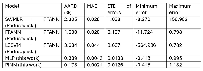
Both MLP and PINN have achieved better numerical performance than the article referenced. Unfortunately, I do not have full access to the article to confirm the architecture or detailed procedure of training the ANNs.

The overall idea of introducing theory or physics into neural networks is that they act as both a guide to learning the right patterns from the data (i.e. the training efficiency should be improved) and learn additional information from the data due to the theoretical model (i.e. expanding into models explainability). While the models will perform effectively on the input space represented in the training set, they might be less likely to perform well outside those bounds. For example, increasing pressure or temperature beyond those bounds included in the training (especially for specific cations and anions). This puts significant limitations on how applicable ANNs could be for designer molecules. However, FT-EoS (as one of the many equations of state available in the literature) was originally developed to combat the issues related to pressure and temperature dependencies of IL densities. While one could just use FT-EoS to calculate densities and elevated temperature and pressure, some initial information is still required (for example, density at room temperature and atmospheric pressure), which again — puts into question how this can be used for designer molecules (unless coupled with some other methods that can obtain these required parameters). One of the ideas of combining ANNs and equations of states (such as FT-EoS) provides the exceptional numerical performance and versatility of ANNs while allowing for expansion of what the input space is compared to the training set due to the equation of state nature (for example temperature and pressure beyond the training set).

From the numerical performance table, PINN performs much better than MLP, which proves that the introduction of physics or theory into the model improves the training procedure and generalisation of the model.

Firstly, let’s look at a plot comparing predicted versus actual values for the density for both PINN and MLP models. We can use the code below to get the predictions for the models.

# Initialize the MLP model with the number of input features from the scaled dataset
model_MLP = MLPModel_torch(dataset['X_scaled'].shape[1])

# Load the pre-trained MLP model parameters from a saved file
model_MLP.load_state_dict(torch.load('./Models/model_MLP.pt'))

# Make predictions with the MLP model on the scaled dataset
y_pred_MLP = pd.DataFrame(
 index=dataset['X_scaled'].index, 
 data=model_MLP(torch.tensor(dataset['X_scaled'].values).float()).cpu().detach().flatten(),
 columns=['ρ / kg/m3'])

# Descale the predicted values to their original scale
y_pred_MLP = descale(y_pred_MLP, scaler['y_shift'], scaler['y_factor'])

# Initialize the PINN model with the number of input features from the scaled dataset
model_PINN = PINNModel_torch(dataset['X_scaled'].shape[1])

# Load the pre-trained PINN model parameters from a saved file
model_PINN.load_state_dict(torch.load('./Models/model_PINN.pt'))

# Make predictions with the PINN model on the scaled dataset
y_pred_PINN = pd.DataFrame(
 index=dataset['X_scaled'].index, 
 data=model_PINN(torch.tensor(dataset['X_scaled'].values).float())[0].cpu().detach().flatten(),
 columns=['ρ / kg/m3'])

# Descale the predicted values to their original scale
y_pred_PINN = descale(y_pred_PINN, scaler['y_shift'], scaler['y_factor'])

And then, we can plot it with the code below:

# Create a new figure using Plotly
figure = go.Figure()

# Generate hover text for MLP predictions with details about each data point
text_MLP = ["Index: {}<br>Dataset ID: {}<br>p: {}<br>T: {}<br>M: {}".format(i, df.loc[i, 'Dataset ID'],
 X.loc[i, 'p / MPa'],
 X.loc[i, 'T / K'],
 X.loc[i, 'M g/mol']) for i in y.index]

# Generate hover text for PINN predictions with details about each data point
text_PINN = ["Index: {}<br>Dataset ID: {}<br>p: {}<br>T: {}<br>M: {}".format(i, df.loc[i, 'Dataset ID'],
 X.loc[i, 'p / MPa'],
 X.loc[i, 'T / K'],
 X.loc[i, 'M g/mol']) for i in y.index]

# Add a scatter plot trace for MLP predictions vs actual values
figure.add_trace(go.Scatter(x=y.values.flatten(), y=y_pred_MLP.values.flatten(),
 mode='markers', name='MLP',
 hovertemplate="Actual: %{x:.4f}<br>Predicted: %{y:.4f}<br>%{text}",
 text=text_MLP))

# Add a scatter plot trace for PINN predictions vs actual values
figure.add_trace(go.Scatter(x=y.values.flatten(), y=y_pred_PINN.values.flatten(),
 mode='markers', name='PINN',
 hovertemplate="Actual: %{x:.4f}<br>Predicted: %{y:.4f}<br>%{text}",
 text=text_PINN))

# Add a line trace representing the perfect prediction line
figure.add_trace(go.Scatter(x=[0.8, 2.8], y=[0.8, 2.8], mode='lines', name='Perfect prediction line'))

# Update the layout of the figure with axis titles and plot title
figure.update_layout(xaxis_title='Actual values', yaxis_title='Predicted values',
 title='Actual versus predicted values for PINN and MLP')

# Save the figure as an HTML file
figure.write_html('./Figures/pred_versus_actual.html')

In Figure 4, one can see how good the predicted versus actual data are. PINN has better performance (i.e., it is closer to the green line representing perfect prediction). All visualisations are available as interative Plotly files on GitHub: Simply click here.

A few sets of data points belong to the same IL and have systematically worse performance for MLP than PINN, as in Figure 5.

Some of those dataset IDs were identified and plotted separately to highlight potential issues. For example, dataset ID 1186, as plotted in Figure 6, is one of those.

MLP predictions are significantly deviated from the actual data, while PINN accurately captured the dependence of density on the temperature (at p = 0.1 MPa). Another example is dataset ID 3931 in Figure 7.

In this case, the predictions are off for MLP at higher pressure (> 80 MPa), particularly for higher temperatures, while PINN performed better. The visualisations above highlight the importance of introducing physics into the black-box models, which allows the right trends and generalisations to be captured.

In physical and computational chemistry, the essence of equations of state is that many of them are mathematically correlated. For example, the solution of one equation of state can often lead to or be used in another equation of state. With this in mind, the parameters obtained in the PINN in this work (υ, ρ0 and k) can be transferable to other areas. For example, the k parameter can be used to derive other thermophysical properties (or help understand, such as isothermal compressibility) through appropriate numerical analysis. ρ0 is an important parameter as it describes density value at room temperature and atmospheric pressure — a valuable parameter in many other equations of state.

Conclusions

I have shown in this article that PINNs can improve the training efficiency and numerical performance of such models compared to MLPs. In this article, a simplistic approach to PINNs was applied. Further expansions are possible; for example, v and k can be treated as a gateway to other thermophysical properties to incorporate in training and evaluation as a density derivative (for example, isobaric expansion or isothermal compressibility). Analysis of obtained parameters included in the output layer of PINN could also be performed; for example, ordinarily, PINNs would have ODEs in their evaluations with appropriate upper and lower bounds of the parameters. Nevertheless, this article aimed to showcase some of the benefits of PINNs.

References

[1] Welcome to the SHAP documentation — SHAP latest documentation

Local Interpretable Model-Agnostic Explanations (lime) — lime 0.1 documentation (lime-ml.readthedocs.io)

Captum · Model Interpretability for PyTorch

[2] [2308.08468] An Expert’s Guide to Training Physics-informed Neural Networks (arxiv.org)

So, what is a physics-informed neural network? — Ben Moseley

Physics-informed machine learning | Nature Reviews Physics

[3] DNN — Tutorial 2 Part I: Physics inspired Machine Learning — UvA DL Notebooks v1.2 documentation (uvadlc-notebooks.readthedocs.io)

mathLab/PINA: Physics-Informed Neural networks for Advanced modeling (github.com)

maziarraissi/PINNs: Physics Informed Deep Learning: Data-driven Solutions and Discovery of Nonlinear Partial Differential Equations (github.com)

[4] Introduction: Ionic Liquids | Chemical Reviews (acs.org)

[5] Extensive Databases and Group Contribution QSPRs of Ionic Liquids Properties. 1. Density | Industrial & Engineering Chemistry Research (acs.org)

[6] kamil2oster/QSPR_PINNs (github.com)

[7] QSPR_PINNs/1. Prepare Data and check literature performance.ipynb at main · kamil2oster/QSPR_PINNs (github.com)

[8] A Fluctuation Equation of State for Prediction of High-Pressure Densities of Ionic Liquids | Scientific Reports (nature.com)

Join thousands of data leaders on the AI newsletter. Join over 80,000 subscribers and keep up to date with the latest developments in AI. From research to projects and ideas. If you are building an AI startup, an AI-related product, or a service, we invite you to consider becoming a sponsor.

Published via Towards AI