


Nothing but NumPy: Understanding & Creating Neural Networks with Computational Graphs from Scratch
Last Updated on May 20, 2020 by Editorial Team
Author(s): Rafay Khan
Understanding new concepts can be hard, especially these days when there is an avalanche of resources with only cursory explanations for complex concepts. This blog is the result of a dearth of detailed walkthroughs on how to create neural networks in the form of computational graphs.
In this blog post, I consolidate all that I have learned as a way to give back to the community and help new entrants. I will be creating common forms of neural networks all with the help of nothing but NumPy.
This blog post is divided into two parts, the first part will be understanding the basics of a neural network and the second part will comprise the code for implementing everything learned from the first part.
Part Ⅰ: Understanding a Neural Network
Let’s dig in
Neural networks are a model inspired by how the brain works. Similar to neurons in the brain, our ‘mathematical neurons’ are also, intuitively, connected to each other; they take inputs(dendrites), do some simple computation on them, and produce outputs(axons).
The best way to learn something is to build it. Let’s start with a simple neural network and hand-solve it. This will give us an idea of how the computations flow through a neural network.
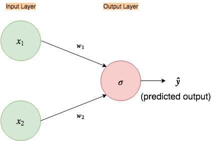
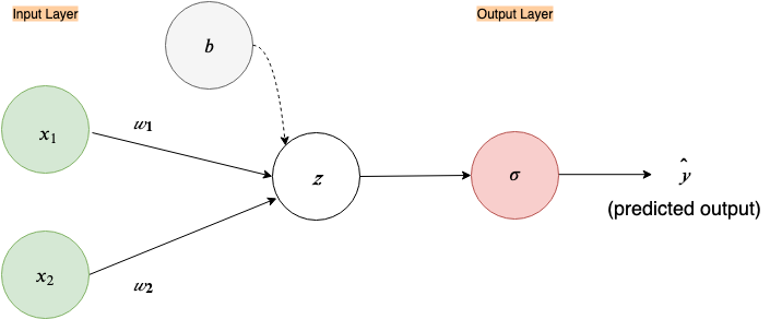
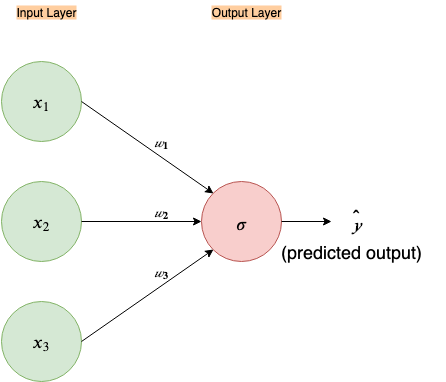
Fig 1. Simple input-output only neural network.
As in the figure above, most of the time you will see a neural network depicted in a similar way. But this succinct and simple looking picture hides a bit of the complexity. Let’s expand it out.
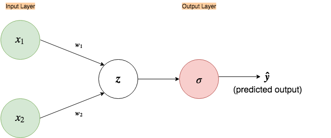
Now, let’s go over each node in our graph and see what it represents.
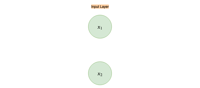
These nodes represent our inputs for our first and second features, x₁ and x₂, that define a single example we feed to the neural network, thus called “Input Layer”

w₁ and w₂ represent our weight vectors (in some neural network literature it is denoted with the theta symbol, θ). Intuitively, these dictate how much influence each of the input features should have in computing the next node. If you are new to this, think of them as playing a similar role to the ‘slope’ or ‘gradient’ constant in a linear equation.
Weights are the main values our neural network has to “learn”. So initially, we will set them to random values and let the “learning algorithm” of our neural network decide the best weights that result in the correct outputs.
Why random initialization? More on this later.

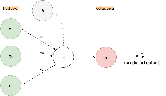
This node represents a linear function. Simply, it takes all the inputs coming to it and creates a linear equation/combination out of them. ( By convention, it is understood that a linear combination of weights and inputs is part of each node, except for the input nodes in the input layer, thus this node is often omitted in figures, like in Fig.1. In this example, I’ll leave it in)
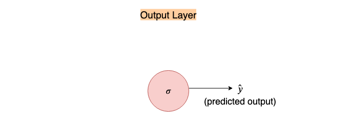
This σ node takes the input and passes it through the following function, called the sigmoid function(because of its S-shaped curve), also known as the logistic function:

Sigmoid is one of the many “activations functions” used in neural networks. The job of an activation function is to change the input to a different range. For example, if z > 2 then, σ(z) ≈ 1 and similarly, if z < -2 then, σ(z) ≈ 0. So, the sigmoid function squashes the output range to (0, 1) (this ‘()’ notation implies exclusive boundaries; never completely outputs 0 or 1 as the function asymptotes, but reaches very close to boundary values)
In our above neural network since it is the last node, it performs the function of output. The predicted output is denoted by ŷ. (Note: in some neural network literature this is denoted by ‘h(θ)’, where ‘h’ is called the hypothesis i.e. this is the hypothesis of the neural network, a.k.a the output prediction, given parameter θ; where θ are weights of the neural networks)
Now that we know what each and everything represents let’s flex our muscles by computing each node by hand on some dummy data.

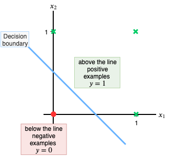
The data above represents an OR gate(output 1 if any input is 1). Each row of the table represents an ‘example’ we want our neural network to learn from. After learning from the given examples we want our neural network to perform the function of an OR gate; given the input features, x₁ and x₂,try to output the corresponding y(also called ‘label’). I have also plotted the points on a 2-D plane so that it is easy to visualize(green crosses represent points where the output(y) is 1 and the red dot represents the point where the output is 0).
This OR-gate data is particularly interesting, as it is linearly separable i.e. we can draw a straight line to separate the green cross from the red dot.
We’ll shortly see how our simple neural network performs this task.
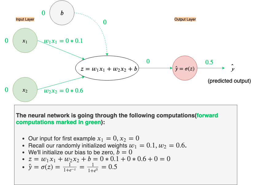
Data flows from left-to-right in our neural network. In technical terms, this process is called ‘forward propagation’; the computations from each node are forwarded to the next node, it is connected to.
Let’s go through all the computations our neural network will perform on given the first example, x₁=0, and x₂=0. Also, we’ll initialize weights w₁and w₂ to w₁=0.1 and w₂=0.6 (recall, these weights a have been randomly selected)
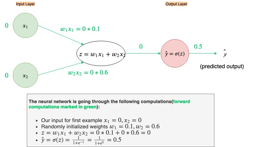
With our current weights, w₁= 0.1 and w₂ = 0.6, our network’s output is a bit far from where we’d like it to be. The predicted output, ŷ, should be ŷ≈0for x₁=0 and x₂=0, right now its ŷ=0.5.
So, how does one tell a neural network how far it is from our desired output? In comes the Loss Function to the rescue.
Loss Function
The Loss Function is a simple equation that tells us how far our neural network’s predicted output(ŷ) is from our desired output(y), for ONE example, only.
The derivative of the loss function dictates whether to increase or decrease weights. A positive derivative would mean decrease the weights and negative would mean increase the weights. The steeper the slope the more incorrect the prediction was.

The Loss function curve depicted in Figure 11 is an ideal version. In real-world cases, the Loss function may not be so smooth, with some bumps and saddles points along the way to the minimum.
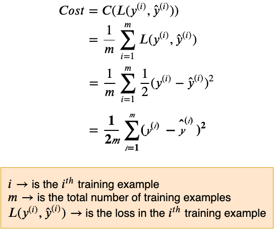
There are many different kinds of loss functions each essentially calculating the error between predicted output and desired output. Here we’ll use one of the simplest loss functions, the squared-error Loss function. Defined as follows:

Taking the square keeps everything nice and positive and the fraction (1/2) is there so that it cancels out when taking the derivative of the squared term (it is common among some machine learning practitioners to leave the fraction out).
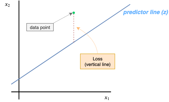
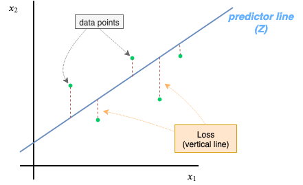
Intuitively, the Squared Error Loss function helps us in minimizing the vertical distance between our predictor line(blue line) and actual data(green dot). Behind the scenes, this predictor line is our z(linear function) node.
Now that we know the purpose of a Loss function let’s calculate the error in our current prediction ŷ=0.5, given y=0

As we can see the Loss is 0.125. Given this, we can now use the derivative of the Loss function to check whether we need to increase or decrease our weights.
This process is called backpropagation, as we’ll be doing the opposite of the forward phase. Instead of going from input to output we’ll track backward from output to input. Simply, backpropagation allows us to figure out how much of the Loss each part of the neural network was responsible for.
To perform backpropagation we’ll employ the following technique: at each node, we only have our local gradient computed(partial derivatives of that node), then during backpropagation, as we are receiving numerical values of gradients from upstream, we take these and multiply with local gradients to pass them on to their respective connected nodes.
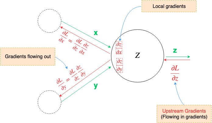
This is a generalization of the chain rule from calculus.
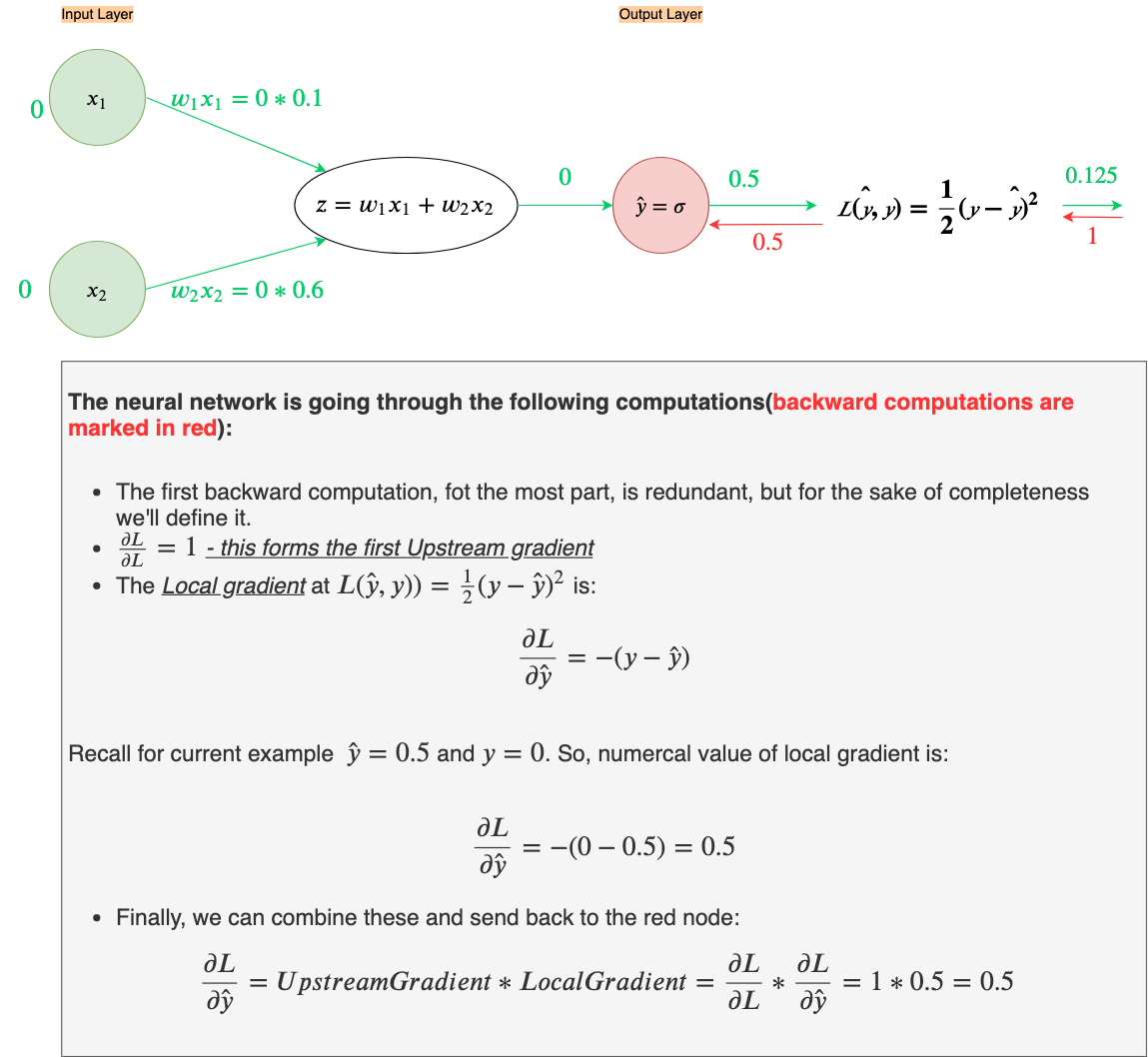
Since ŷ(predicted label) dictates our Loss and y(actual label) is constant, for a single example, we will take the partial derivative of Loss with respect to ŷ

Since the backpropagation steps can seem a bit complicated I’ll go over them step by step:
For the next calculation, we’ll need the derivative of the sigmoid function, since it forms the local gradient of the red node. Let’s derive that.


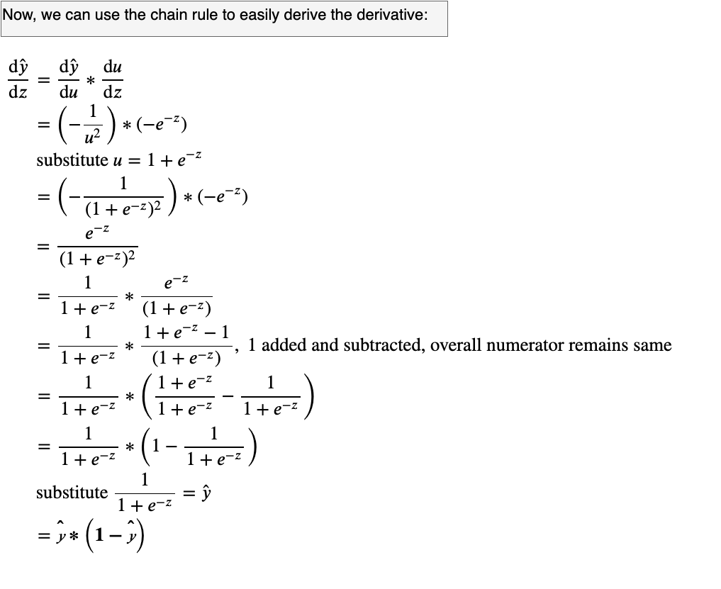
Let’s use this in the next backward calculation

The backward computations should not propagate all the way to inputs as we don’t want to change our input data(i.e. red arrows should not go to green nodes). We only want to change the weights associated with inputs.

Notice something weird? The derivatives to the Loss with respect to the weights,w₁ & w₂, are ZERO! We can’t increase or decrease the weights if their derivatives are zero. So then, how do we get our desired output in this instance if we can’t figure out how to adjust the weights? The key thing to note here is that the local gradients (∂z/∂w₁ and ∂z/∂w₂) are x₁ and x₂, both of which, in this example, happens to be zero (i.e. provide no information)
This brings us to the concept of bias.
Bias
Recall equation of a line from your high school days.
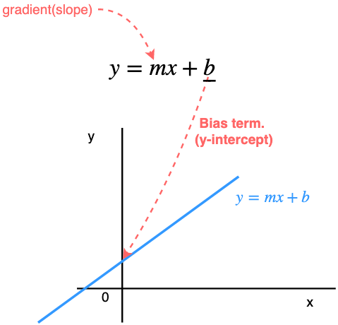
Here b is the bias term. Intuitively, the bias tells us that all outputs computed with x(independent variable) should have an additive bias of b.So, when x=0(no information coming from the independent variable) the output should be biased to just b.
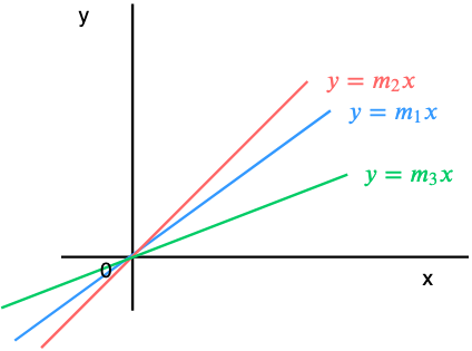
Note that without the bias term a line can only pass through the origin(0, 0) and the only differentiating factor between lines would then be the gradient m.
So, using this new information let’s add another node to a neural network; the bias node. (In neural network literature, every layer, except the input layer, is assumed to have a bias node, just like the linear node, so this node is also often omitted in figures.)
Now let’s do a forward propagation with the same example, x₁=0, x₂=0, y=0 and let’s set bias, b=0 (initial bias is always set to zero, rather than a random number), and let the backpropagation of Loss figure out the bias.
Well, the forward propagation with a bias of “b=0” didn’t change our output at all, but let’s do the backward propagation before we make our final judgment.
As before let’s go through backpropagation in a step by step manner.


Hurrah! we just figured out how much to adjust the bias. Since the derivative of bias(∂L/∂b) is positive 0.125, we will need to adjust the bias by moving in the negative direction of the gradient(recall the curve of the Loss function from before). This is technically called gradient descent, as we are “descending” away from the sloping region to a flat region using the direction of the gradient. Let’s do that.

Now, that we’ve slightly adjusted the bias to b=-0.125, let’s test if we’ve done the right thing by doing a forward propagation and checking the new Loss.
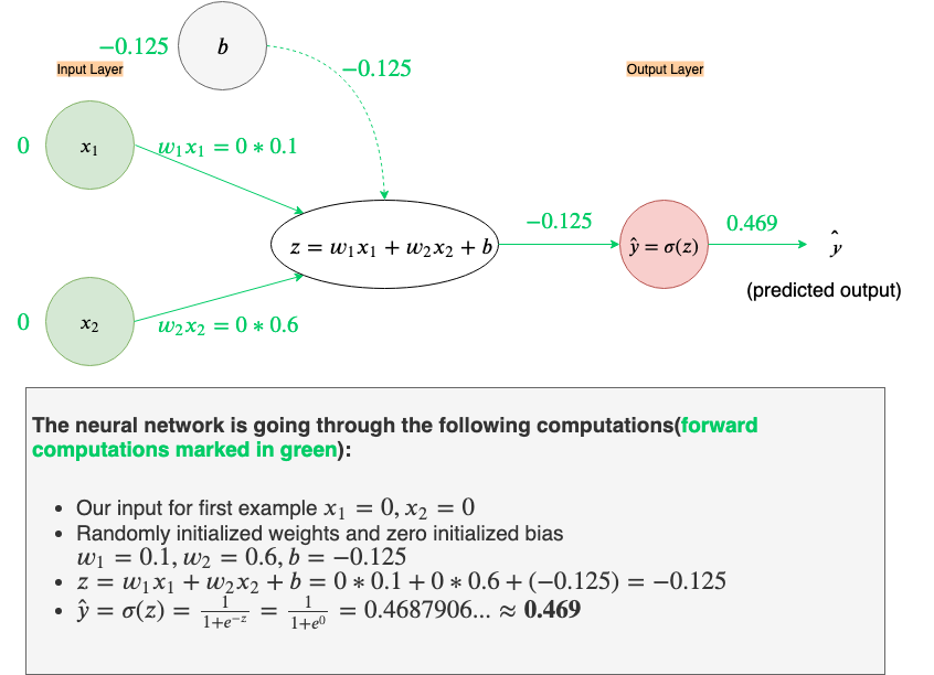

Now our predicted output is ŷ≈0.469(rounded to 3 decimal places), that’s a slight improvement from the previous 0.5 and Loss is down from 0.125 to around 0.109. This slight correction is something that the neural network has ‘learned’ just by comparing its predicted output with the desired output, y, and then moving in the direction opposite of the gradient. Pretty cool, right?
Now you may be wondering, this is only a small improvement from the previous result and how do we get to the minimum Loss. Two things come into play: a) how many iterations of ‘training’ we perform (each training cycle is forward propagation followed by backward propagation and updating the weights through gradient descent). b) the learning rate.
Learning rate??? What’s that? Let’s talk about it.
Learning Rate
Recall, how we calculated the new bias, above, by moving in the direction opposite of the gradient(i.e. gradient descent).

Notice that when we updated the bias we moved 1 step in the opposite direction of the gradient.
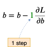
We could have moved 0.5, 0.9, 2, 3 or whatever fraction of steps we desired in the opposite direction of the gradient. This ‘number of steps’ is what we define as the learning rate, often denoted with α(alpha).

Learning rate defines how quickly we reach the minimum loss. Let’s visualize below what the learning rate is doing:
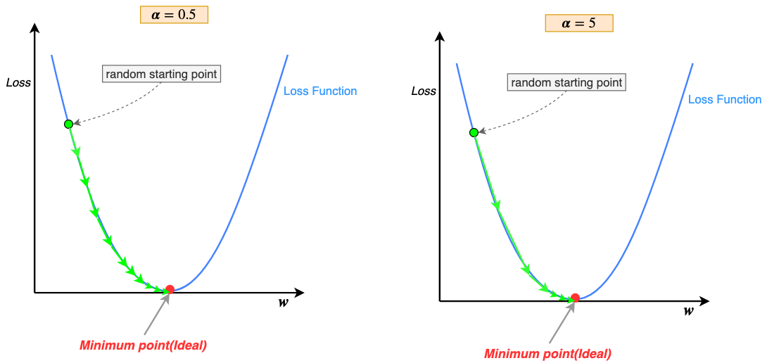
As you can see with a lower learning rate(α=0.5) our descent along the curve is slower and we take many steps to reach the minimum point. On the other hand, with a higher learning rate(α=5) we take much bigger steps and reach the minimum point much faster.
The keen-eyed may have noticed that gradient descent steps(green arrows) keep getting smaller as we get closer and closer to the minimum, why is that? Recall, that the learning rate is being multiplied by the gradient at that point along the curve; as we descend away from sloping regions to flatter regions of the u-shaped curve, near the minimum point, the gradient keeps getting smaller and smaller, thus the steps also get smaller. Therefore, changing the learning rate during training is not necessary(some variations of gradient descent start with a high learning rate to descend quickly down the slope and then reduce it gradually, this is called “annealing the learning rate”)
So what’s the takeaway? Just set the learning rate as high possible and reach the optimum loss quickly. NO. Learning rate can be a double-edged sword. Too high a learning rate and the parameters(weights/biases) don’t reach the optimum instead start to diverge away from the optimum. To small a learning rate and the parameters take too long to converge to the optimum.
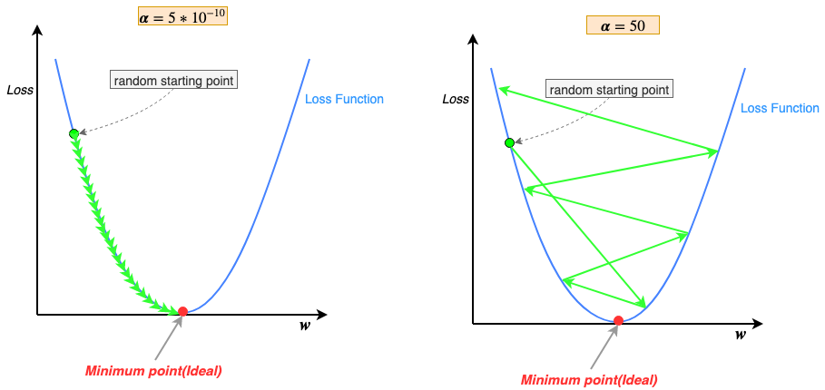
Small learning rate(α=5*10⁻¹⁰) resulting is numerous steps to reach the minimum point is self-explanatory; multiply gradient with a small number(α) results in a proportionally small step.
Large learning rate(α=50) causing gradient descent to diverge may be confounding, but the answer is quite simple; note that at each step gradient descent approximates its path downward by moving in straight lines(green arrows in the figures), in short, it estimates its path downwards. When the learning rate is too high we force gradient descent to take larger steps. Larger steps tend to overestimate the path downwards and shoot past the minimum point, then to correct the bad estimate gradient descent tries to move towards the minimum point but again overshoots past the minimum due to the large learning rate. This cycle of continuous overestimates eventually cause the results to diverge(Loss after each training cycle increase, instead of decrease).
Learning rate is what’s called a hyper-parameter. Hyper-parameters are parameters that the neural network can’t essentially learn through backpropagation of gradients, they have to be hand-tuned according to the problem and its dataset, by the creator of the neural network model. (The choice of the Loss function, above, is also hyper-parameter)
In short, the goal is not the find the “perfect learning rate ” but instead a learning rate large enough so that the neural network trains successfully and efficiently without diverging.
So, far we’ve only used one example(x₁=0 and x₂=0) to adjust our weights and bias(actually, only our bias up till now🙃) and that reduced the loss on one example from our entire dataset(OR gate table). But we have more than one example to learn from and we want to reduce our loss across all of them. Ideally, in one training iteration, we would like to reduce our loss across all the training examples. This is called Batch Gradient Descent(or full batch gradient descent), as we use the entire batch of training examples per training iteration to improve our weights and biases. (Others forms are mini-batch gradient descent, where we use a subset of the data set in each iteration and stochastic gradient descent, where we only use one example per training iteration as we’ve done so far).
A training iteration where the neural network goes through all the training examples is called an Epoch. If using mini-batches than an epoch would be complete after the neural network goes through all the mini-batches, similarly for stochastic gradient descent where a batch is just one example.
Before we proceed further we need to define something called a Cost Function.
Cost Function
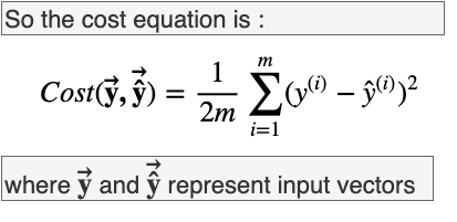
When we perform “batch gradient descent” we need to slightly change our Loss function to accommodate not just one example but all the examples in the batch. This adjusted Loss function is called the Cost Function.
Also, note that the curve of the Cost Function is similar to the curve of the Loss function(same U-Shape).
Instead of calculating the Loss on one example the cost function calculates average Loss across ALL the examples.
Intuitively, the Cost function is expanding out the capability of the Loss function. Recall, how the Loss function was helping to minimize the vertical distance between a single data point and the predictor line(z). The Cost function is helping to minimize the vertical distance(Squared Error Loss) between multiple data points, concurrently.
During batch gradient descent we’ll use the derivative of the Cost function, instead of the Loss function, to guide our path to minimum cost across all examples. (In some neural network literature, the Cost Function is at times also represented with the letter ‘J’.)
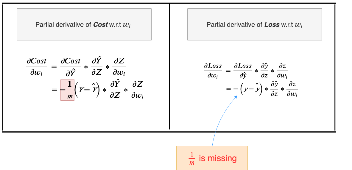
Let’s take a look at how the derivative equation of the Cost function differs from the plain derivative of the Loss function.
The derivative of Cost Function
Taking the derivative of this Cost function, which takes vectors as inputs and sums them, can be a bit dicey. So, let’s start out on a simple example before we generalize the derivative.
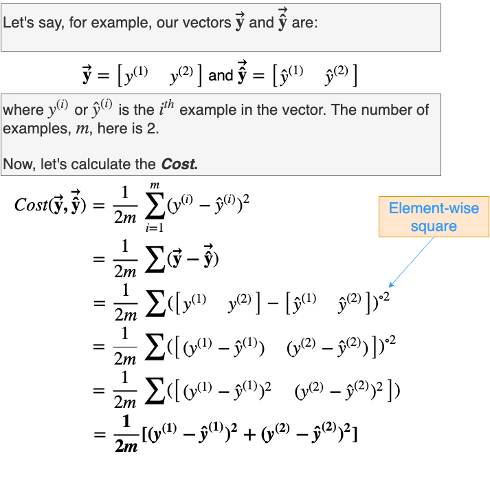
Nothing new here in the calculation of the Cost. Just as expected the Cost, in the end, is the average of the Loss, but the implementation is now vectorized(we performed vectorized subtraction followed by element-wise exponentiation, called Hadamard exponentiation). Let’s derive the partial derivatives.
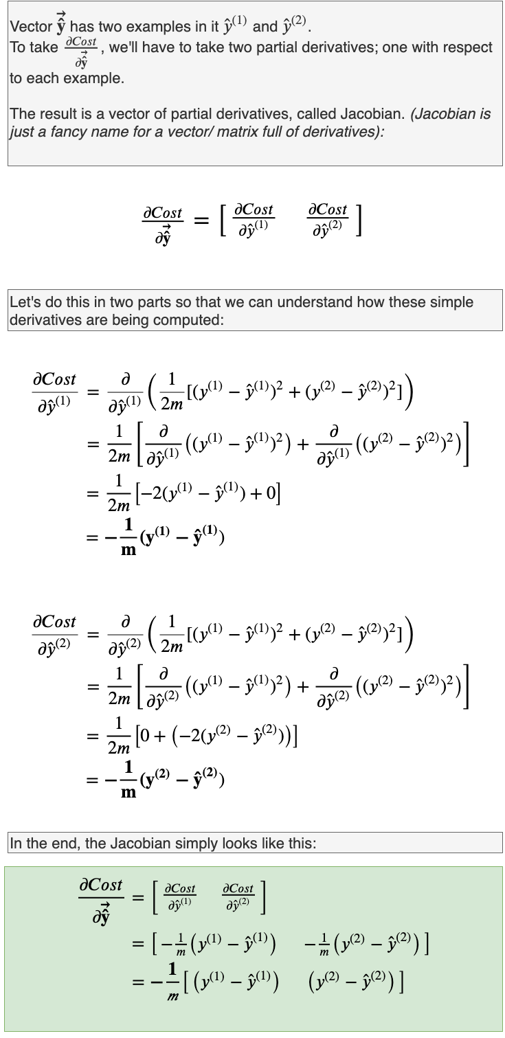
From this, we can generalize the partial derivative equation.
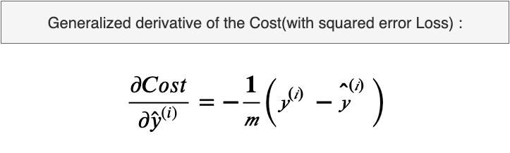
Right now we should take a moment to note how the derivative of the Loss is different for the derivative of the Cost.
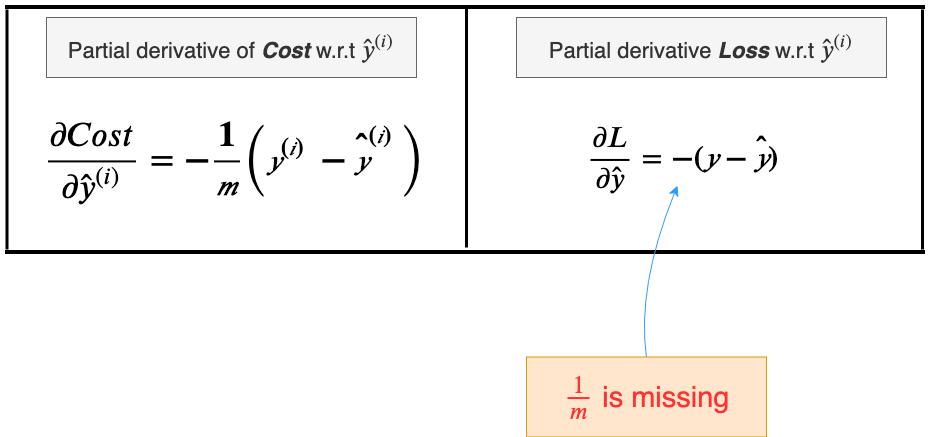
We’ll later see how this small change manifests itself in the calculation of the gradient.
Back to batch gradient descent.
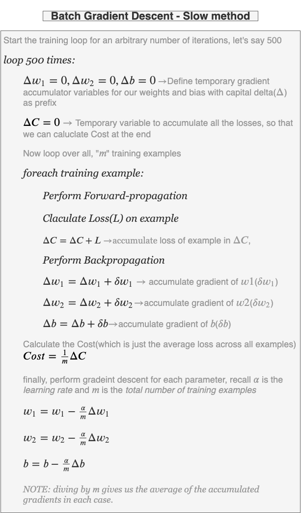
There are two ways to perform batch gradient descent:
1. For each training iteration create separate temporary variables(capital deltas, Δ) that will accumulate the gradients(small deltas, δ) for the weights and biases from each of the “m” examples in our training set, then at the end of the iteration update the weights using the average of the accumulated gradients. This is a slow method. (for those familiar time complexity analysis you may notice that as the training data set grows this becomes a polynomial-time algorithm, O(n²))
2. The quicker method is similar to above but instead uses vectorized computations to calculate all the gradients for all the training examples in one go, so the inner loop is removed. Vectorized computations run much quicker on computers. This is the method employed by all the popular neural network frameworks and the one we’ll follow for the rest of this blog.
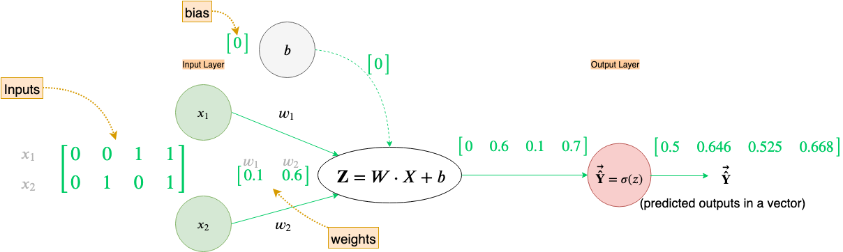
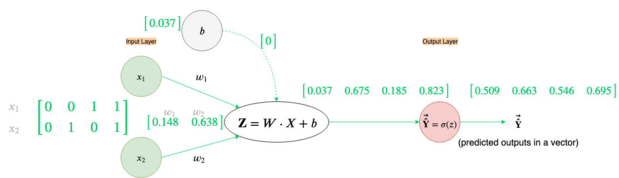
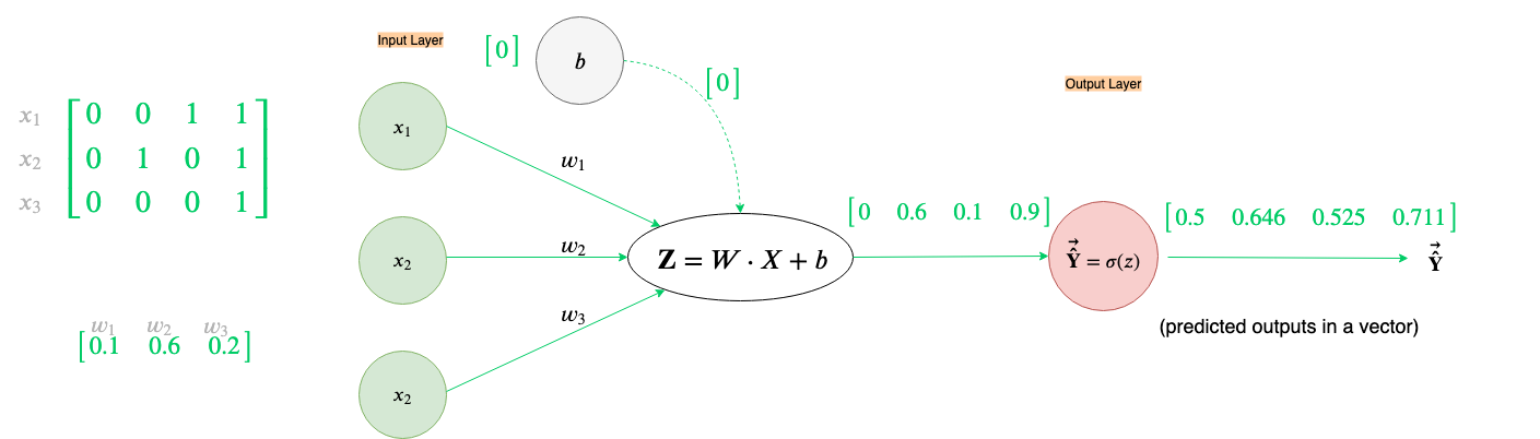
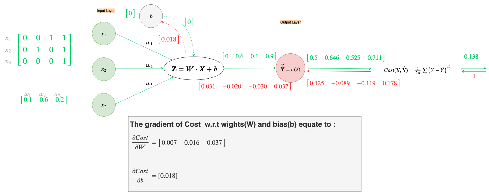
For vectorized computations, we’ll make an adjustment to the “Z” node of the neural network computation graph and use the Cost function instead of the Loss function.
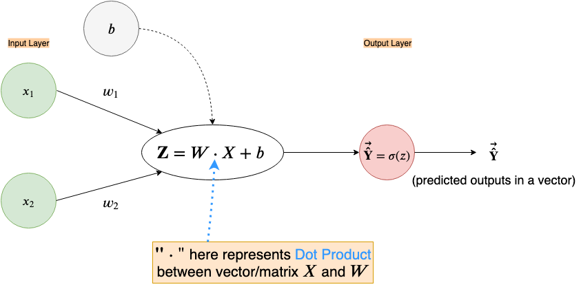
Note that in the figure above we take dot-product between W and X which can be either an appropriate size matrix or vector. The bias, b, is still a single number(a scalar quantity) here and will be added to the output of the dot product in an element-wise fashion. The predicted output will not be just a number, but instead a vector, Ŷ, where each element is the predicted output of their respective example.
Let’s set up out data(X, W, b & Y) before doing forward and backward propagation.
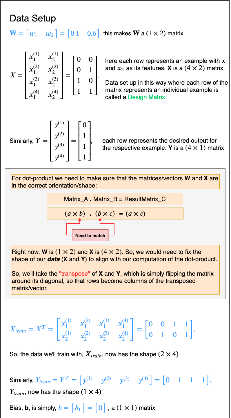
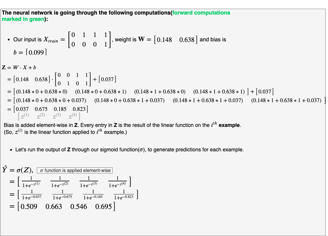
We are now finally ready to perform forward and backward propagation using Xₜᵣₐᵢₙ, Yₜᵣₐᵢₙ, W, and b.
(NOTE: All the results below are rounded to 3 decimal points, just for brevity)
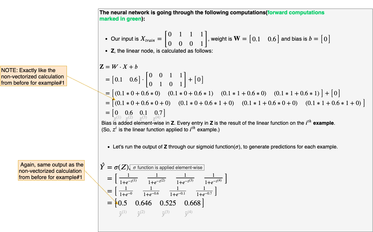
How cool is that we calculated all the forward propagation steps for all the examples in our data set in one go, just by vectorizing our computations.
We can now calculate the Cost on these output predictions. (We’ll go over the calculation in detail, to make sure there is no confusion)
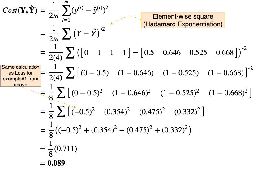
Our Cost with our current weights, W, turns out to be 0.089. Our Goal now is to reduce this cost using backpropagation and gradient descent. As before we’ll go through backpropagation in a step by step manner

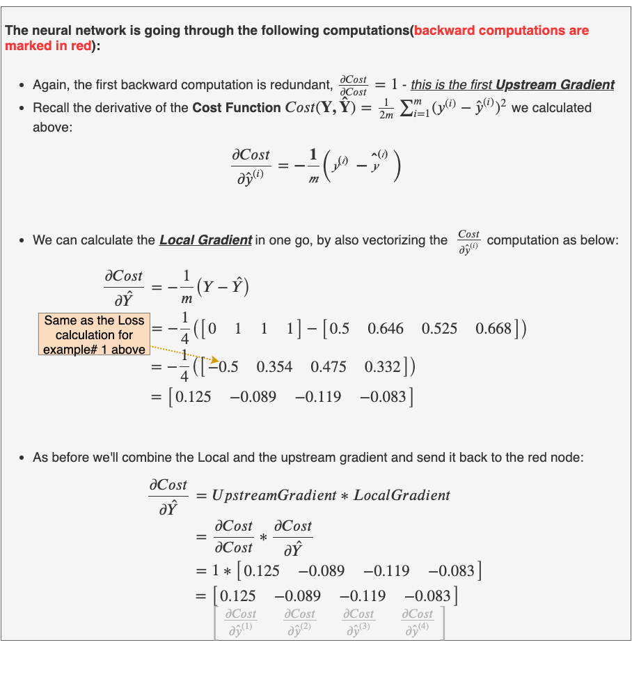

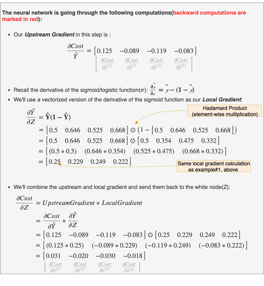

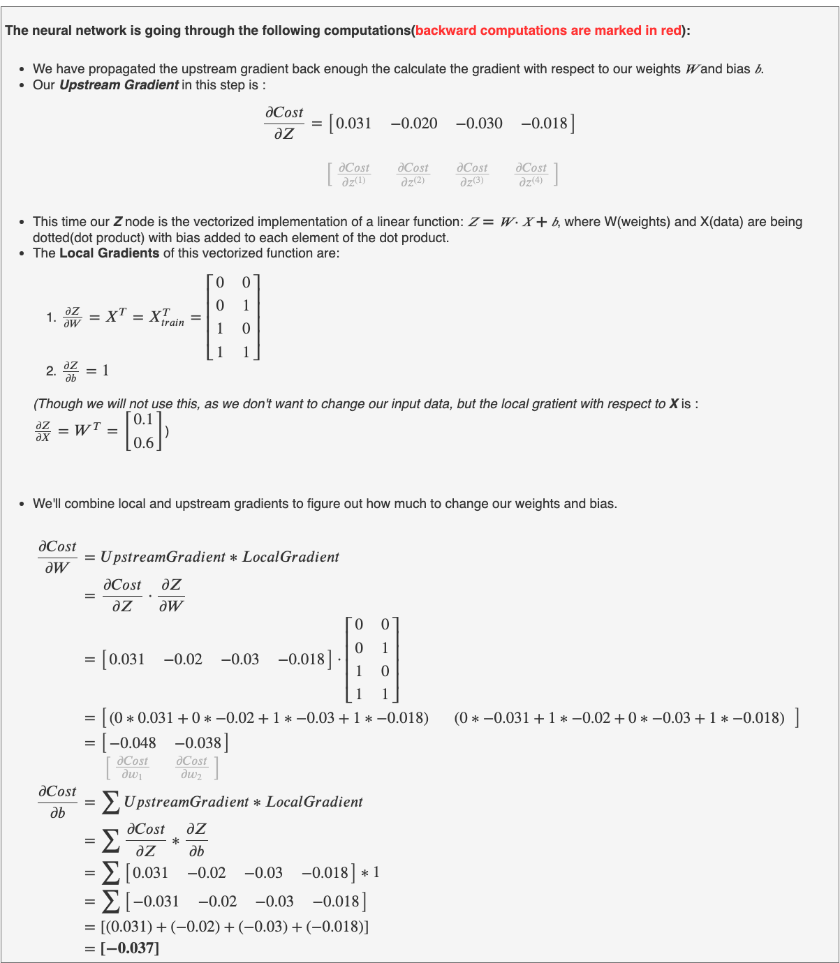
Voila, we used a vectorized implementation of batch gradient descent to calculate all the gradients in one go.
(Those with a keen eye may be wondering how are the local gradients and the final gradients are being calculated in this last step. Don’t worry, I’ll explain the derivation of the gradients in this last step, shortly. For now, its suffice to say that the gradients defined in this last step are an optimization over the naive way of calculating ∂Cost/∂W and ∂Cost/∂b)
Let’s update the weights and bias, keeping learning rate same as the non-vectorized implementation from before i.e. α=1.

Now that we have updated the weights and bias lets do a forward propagation and calculate the new Cost to check if we’ve done the right thing.

So, we reduced our Cost(Average Loss across all examples) from an initial Cost of around 0.089 to 0.084. We will need to do multiple training iterations before we can converge to a low Cost.
At this point, I would recommend that you perform backpropagation step yourself. The result of that should be (rounded to 3 decimal places): ∂Cost/∂W = [-0.044, -0.035] and ∂Cost/∂b = [-0.031].
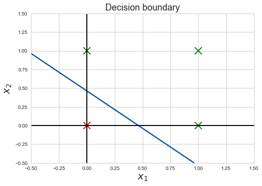
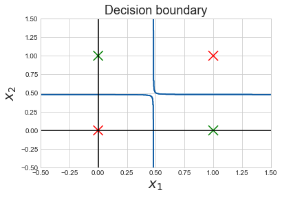
Recall, before we trained the neural network, how we predicted the neural network can separate the two classes in Figure 9, well after about 5000 Epochs(full batch training iterations) Cost steadily decreases to about 0.0005 and we get the following decision boundary :
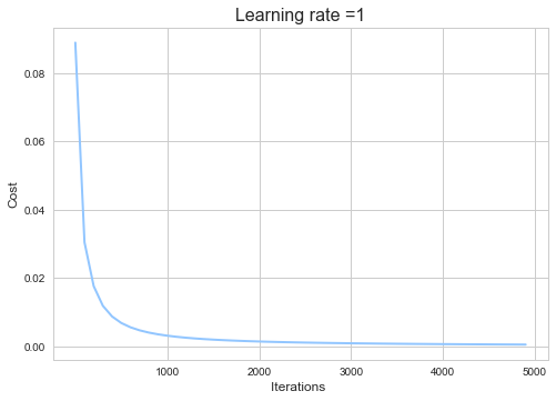
The Cost curve is basically the value of Cost plotted after a certain number of iterations(epochs). Notice that the Cost curve flattens after about 3000 epochs this means that the weights and bias of the neural network have converged, so further training will only slightly improve our weights and bias. Why? Recall the u-shaped Loss curve, as we descend closer and closer the minimum point(flat region) the gradients become smaller and smaller thus the steps gradient descent takes are very small.
The Decision Boundary shows at the line along which the decision of the neural network changes from one output to the other. We can better visualize this by coloring the area below and above the decision boundary.
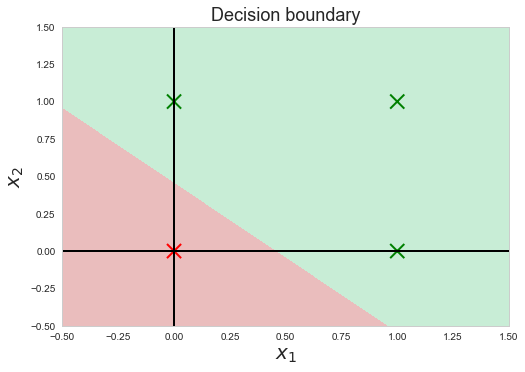
This makes it much clearer. The red shaded area is the area below the decision boundary and everything below the decision boundary has an output( ŷ) of 0. Similarly, everything above the decision boundary, shaded green, has an output of 1. In conclusion, our simple neural network has learned a decision boundary by looking at the training data and figuring out how to separate its two output classes(y=1 and y=0)🙌. Now the output neuron fires up🔥(produces 1) whenever x₁ or x₂ or both are 1.
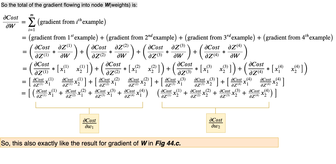
Now would be a good time to see how the “1/m” (“m” is the total number of examples in the training dataset) in the Cost function manifested in the final calculation of the gradients.
From this, the most important point to know is that the gradient that is used to update our weights, using the Cost function, is the average of all the gradients calculated during a training iteration; same applies to bias. You may want to confirm this yourself by checking the vectorized calculations yourself.
Taking the average of all the gradients has some benefits. Firstly, it gives us a less noisy estimate of the gradient. Second, the resultant learning curve is smooth helping us easily determine if the neural network is learning or not. Both of these features come in very handy when training neural networks on much trickier datasets, such as those with wrongly labeled examples.
This is great and all but how did you calculate the gradients ∂Cost/∂W and ∂Cost/∂b ?
Neural network guides and blog posts I learned from often omitted complex details or gave very vague explanations for them. Not in this blog we’ll go over everything leaving no stone unturned.
First, we’ll tackle ∂Cost/∂b. Why did we sum the gradients?
To explain this I employ our computational graph technique on three very simple equations.
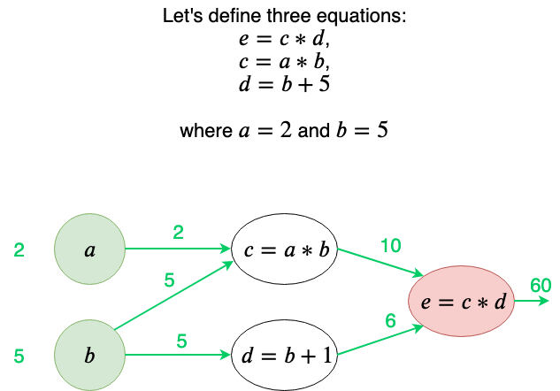
I am particularly interested in the b node, so let’s do backpropagation on this.
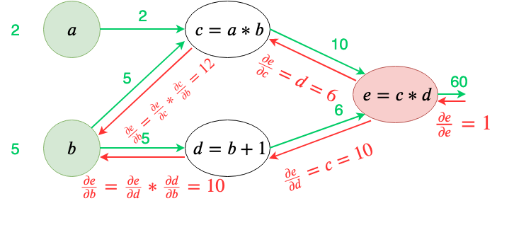
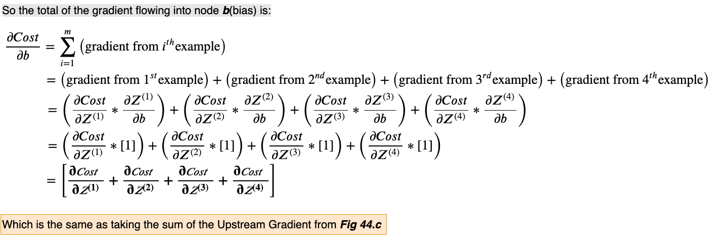
Note that the b node is receiving gradients from two other nodes. So the total of the gradients flowing into node b is the sum of the two gradients flowing in.

From this example, we can generalize the following rule: Sum all the incoming gradients to a node, from all the possible paths.
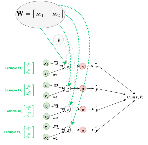
Let’s visualize how this rule is used in the calculation of the bias. Our neural network can be seen as doing independent calculations for each of our examples but using shared parameters for weights and bias, during a training iteration. Below bias(b) is visualized as a shared parameter for all individual calculations our neural network performs.
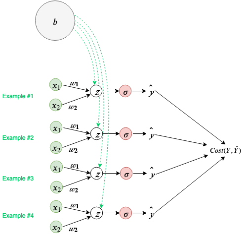
Following the general rule defined above, we will sum all the incoming gradients from all the possible paths to the bias node, b.
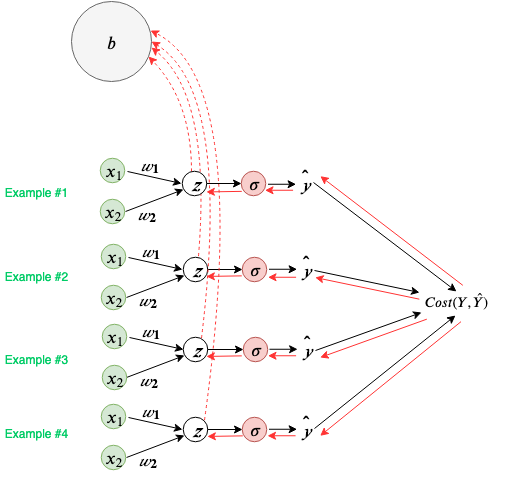
Since the ∂Z/∂b (local gradient at the Z node) is equal to 1, the total gradient at b is the sum of gradients from each example with respect to the Cost.
Now that we’ve got derivative of the bias figured out let’s move on to derivative of weights, and more importantly the local gradient with respect to weights.
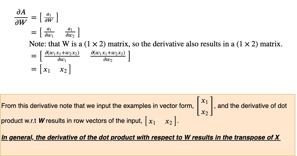
How is the local gradient(∂Z/∂W) equal to transpose of the input training data(X_train)?
This can be answered in a similar way to the above calculation for bias, but the main complication here is the calculating the derivative of the dot product between the weight matrix(W) and the data matrix(Xₜᵣₐᵢₙ), which forms our local gradient.

This derivative of the dot product is a bit complicated as we are no longer working with scalar quantities, instead, both W and X are matrices and the result of W⋅ X is also a matrix. Let’s dive a bit deeper using a simple example first and then generalizing from it.
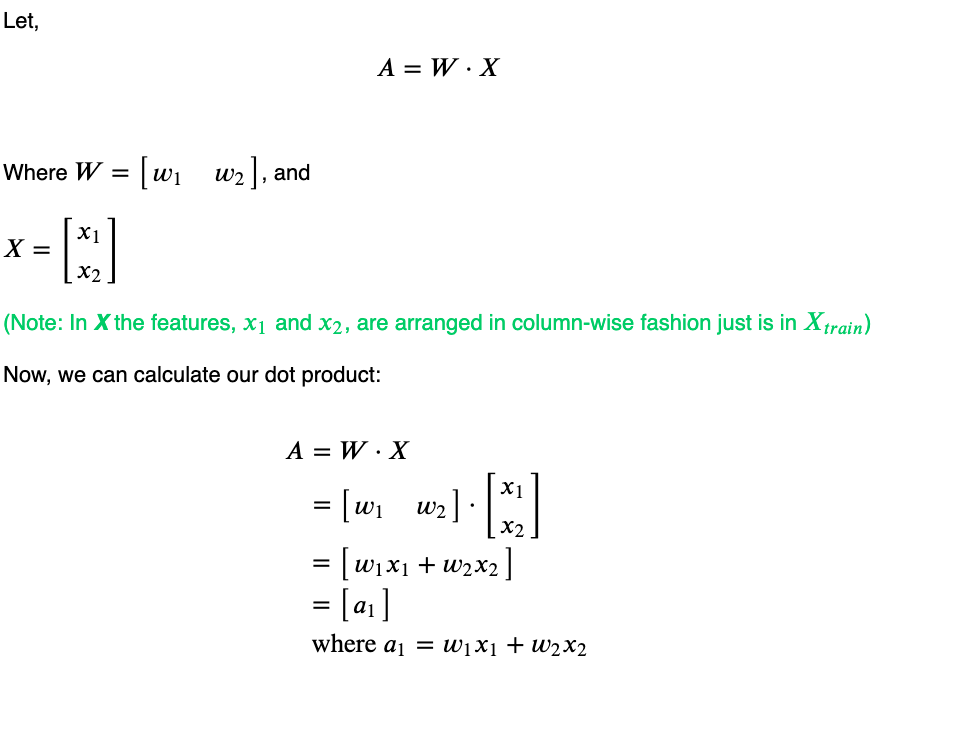
Let’s calculate the derivative of the A with respect to W.
Let us visualize this in case of a training iteration where multiple examples are being processed at the same time. (Note that input examples are column vectors.)
Just as the bias (b) was being shared across each calculation in a training iteration, weights (W) are also being shared. We can also visualize the gradient flowing back to the weights, as follows(note that the local derivative of each example w.r.t to W results in a row vector of the input example i.e. transpose of input):
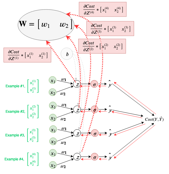
Again, following the general rule defined above, we will sum all the incoming gradients from all the possible paths to the weights node, W.
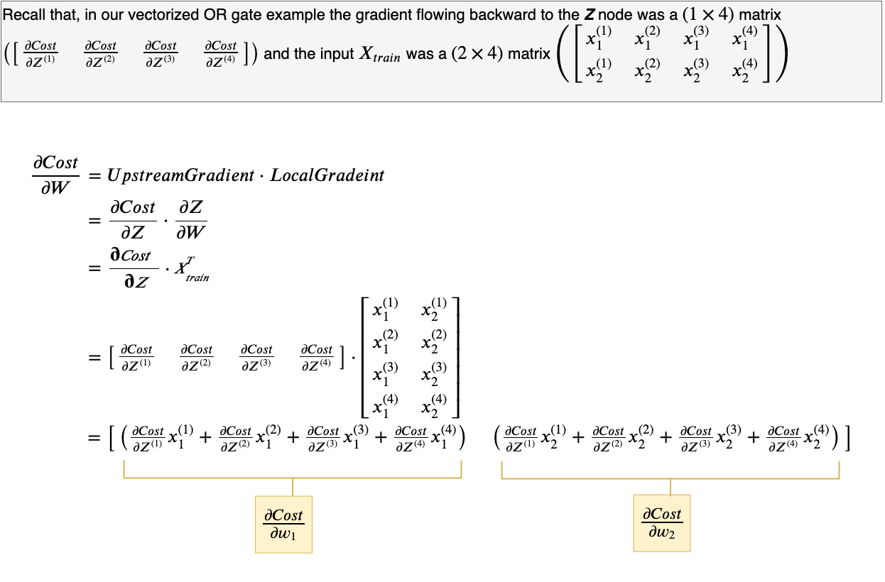
Up till now what we’ve done to calculate, ∂Cost/∂W, though is correct and serves as a good explanation however, it is not an optimized calculation. We can vectorize this calculation, too. Let’s do that next
Is there an easier way of figuring this out, without the math?
Yes! Use dimension analysis.
In our OR gate example we know that the gradient flowing into node Z is a (1 × 4) matrix, Xₜᵣₐᵢₙ is a (2 × 4) matrix and the derivative of Cost with respect to the W needs to be of the same size as W, which is (1 × 2). So, the only way to generate a (1 × 2) matrix would be to take the dot product of between Z and transpose of Xₜᵣₐᵢₙ.

Similarly, knowing that bias, b, is a simple (1 × 1) matrix and the gradient flowing into node Z is (1 × 4), using dimension analysis we can be sure that the gradient of Cost w.r.t b, also needs to be a (1 × 1) matrix. The only way we can achieve this, given the local gradient(∂Z/∂b) is just equal to 1, is by summing up the upstream gradient.
On a final note when deriving derivative expressions work on small examples and then generalize from there. For example here, while calculating the derivative of the dot product w.r.t to W, we used a single column vector as a test case and generalized from there, if we would have used the entire data matrix then the derivative would have resulted in a (4 × 1 × 2) tensor (multidimensional matrix), calculation on which can get a bit hairy.
Before concluding this section lets go over a slightly more complicated example.

Figure 62, above, represents an XOR gate data. Looking at it note that the label, y, is equal to 1 only when one of the values x₁ or x₂ is equal to 1, not both. This makes it a particularly challenging dataset as the data is not linearly separable, i.e. there is no single straight line decision boundary that can successfully separate the two classes(y=1 and y=0) in the data. XOR used to be the bane of earlier forms of artificial neural networks.
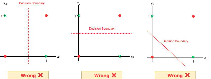
Recall that our current neural network was successful only because it could figure out the straight line decision boundary that could successfully separate the two classes of the OR gate dataset. A straight line won’t cut it here. So, how do we get a neural network to figure this one out?
Well, we can do two things:
- Amend the data itself, so that in addition to features x₁ and x₂ a third feature provides some additional information to help the neural network decide on a good decision boundary. This process is called feature engineering.
- Change the architecture of the neural network, making it deeper.
Let’s go over both and see which one is better.
Feature Engineering
Let’s look at a dataset similar looking to the XOR data that will help us in making an important realization.

The data in Figure 64 is exactly like the XOR data except each data point is spread out in different quadrants. Notice that in the 1ˢᵗ and 3ʳᵈ quadrant all the values are positive and in the 2ⁿᵈ and 4ᵗʰ all the values are negative.

Why is that? In the 1ˢᵗ and 3ʳᵈ quadrants the signs of values are being squared, while in the 2ⁿᵈ and 4ᵗʰ quadrants the values are a simple product between a negative and positive number resulting in a negative number.
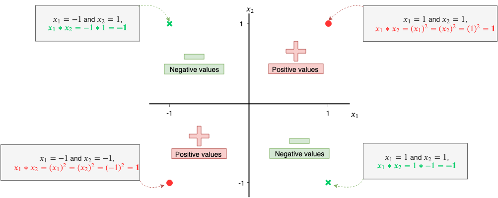
So this gives us a pattern to work with using the product of two features. We can even see a similar pattern in the XOR data, where each quadrant can be identified in a similar way.

Therefore, a good third feature, x₃, would be the product of features x₁ and x₂(i.e. x₁*x₂).
Product of features is called a feature cross and results in a new synthetic feature. Feature crosses can be either the feature itself(eg. x₁², x₁³,…), a product of two or more features(eg. x₁*x₂, x₁*x₂*x₃, …) or even a combination of both(eg. x₁²*x₂). For example, in a housing dataset where the input features are the width and length of houses in yards and label is the location of the house on the map, a better predictor for this location could be the feature cross between width and length of houses, giving us a new feature of “size of house in square yards”.
Let’s add the new synthetic feature to our training data, Xₜᵣₐᵢₙ.

Using this feature cross we can now successfully learn a decision boundary without changing the architecture of the neural network significantly. We only need to add an input node for x₃ and a corresponding weight(randomly set to 0.2) to the input layer.
Given below is the first training iteration of the neural network, you may go through the computations yourself and confirm them as they make for a good exercise. Since we are already familiar with this neural network architecture, I will not go through all the computations in a step-by-step by step manner, as before.
(All calculations below are rounded to 3 decimal places)

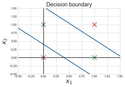
After 5000 epochs, the learning curve, and the decision boundary look as follows:

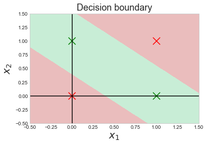
As before, to visualize better we can shade the regions where the decision of the neural network changes from one to the other.

Note that feature engineering allowed us to create a decision boundary that is nonlinear. How did it do that? We just need to take a look at what function the Z node is computing.
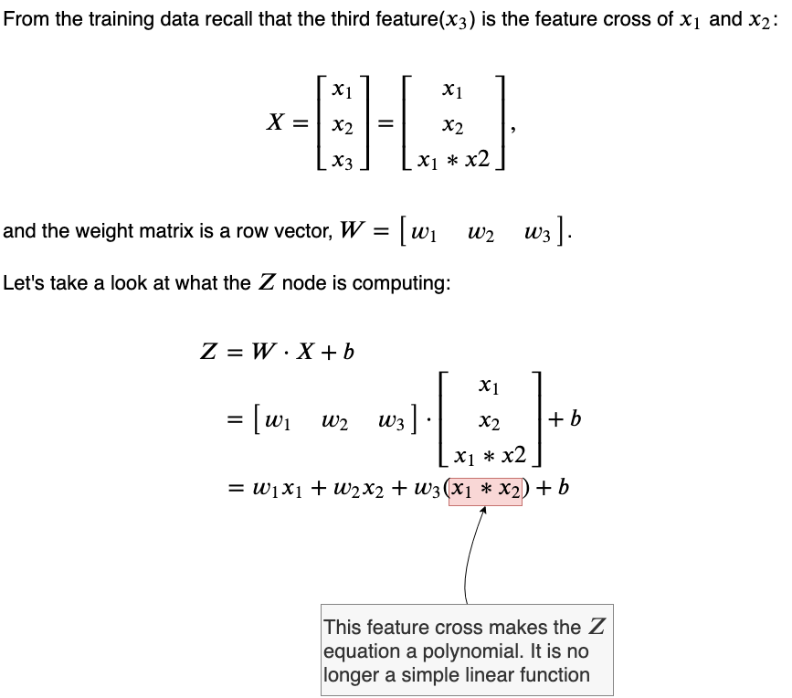
Thus, feature cross helped us to create complex non-linear decision boundary.
This is a very powerful idea!
Changing Neural Network Architecture
This is the more interesting approach as it allows us to bypass the feature engineering ourselves and lets the neural network figure out the feature crosses itself!
Let’s take a look at the following neural network:
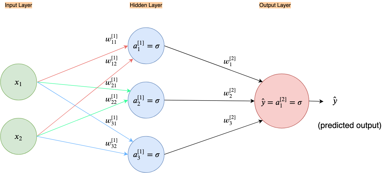
So we’ve added a bunch of new nodes in the middle of our neural network architecture from the OR gate example, keeping the input layer and the output layer the same. This column of new nodes in the middle is called a hidden layer. Why hidden layer? Because after defining it we don’t have any direct control over how the neurons in the hidden layers learn, unlike the input and output layer which we can change by changing the data; also since the hidden layers neither constitute as the output or the input of the neural network they are in essence hidden from the user.
We can have an arbitrary number of hidden layers with an arbitrary number of neurons in each layer. This structure needs to be defined by the creator of the neural network. Thus, the number of hidden layers and the number of neurons in each of the layers are also hyper-parameters. The more hidden layers we add the deeper our neural network architecture becomes and the more neurons we add in the hidden layers the wider the network architecture becomes. The depth of a neural net model is where the term “Deep learning” comes from.
The architecture in Figure 77 with one hidden layer of three sigmoid neurons, was selected after some experimentation.
Since this is a new architecture I’ll go over the computations step-by-step.
First, let’s expand out the neural network.
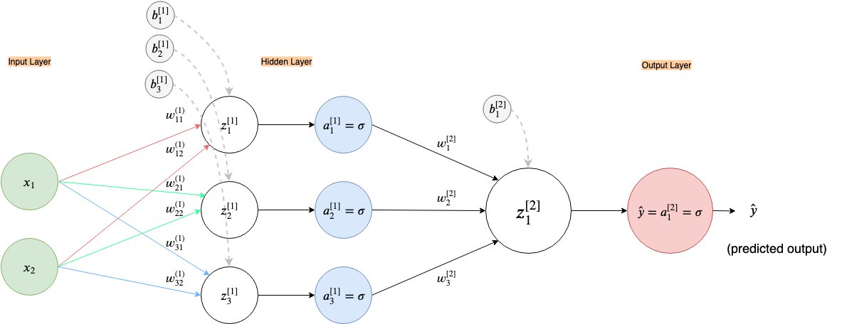
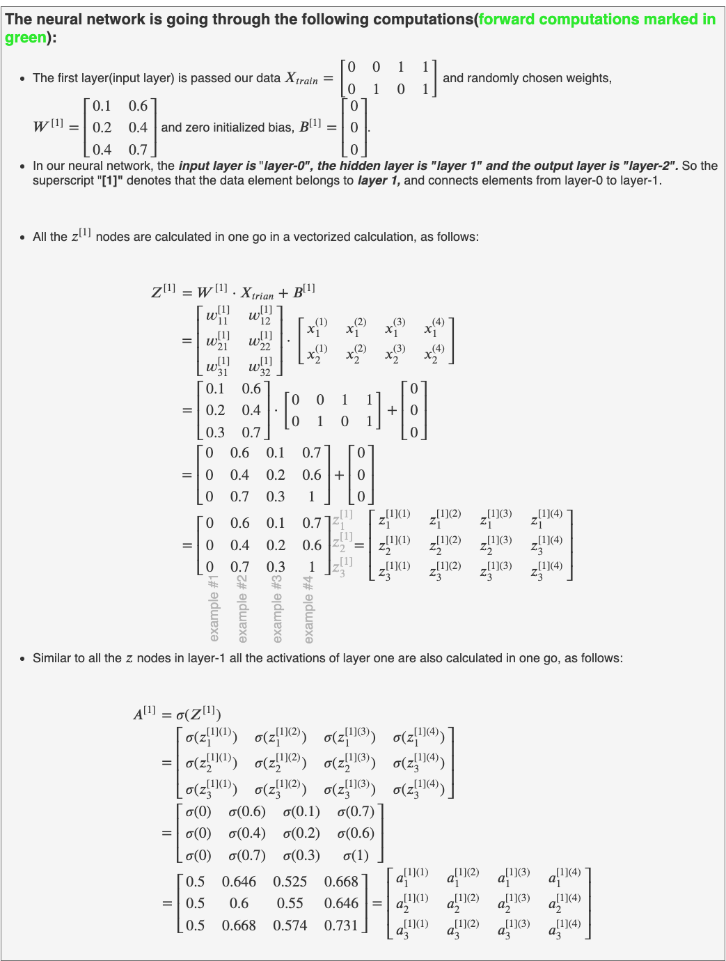
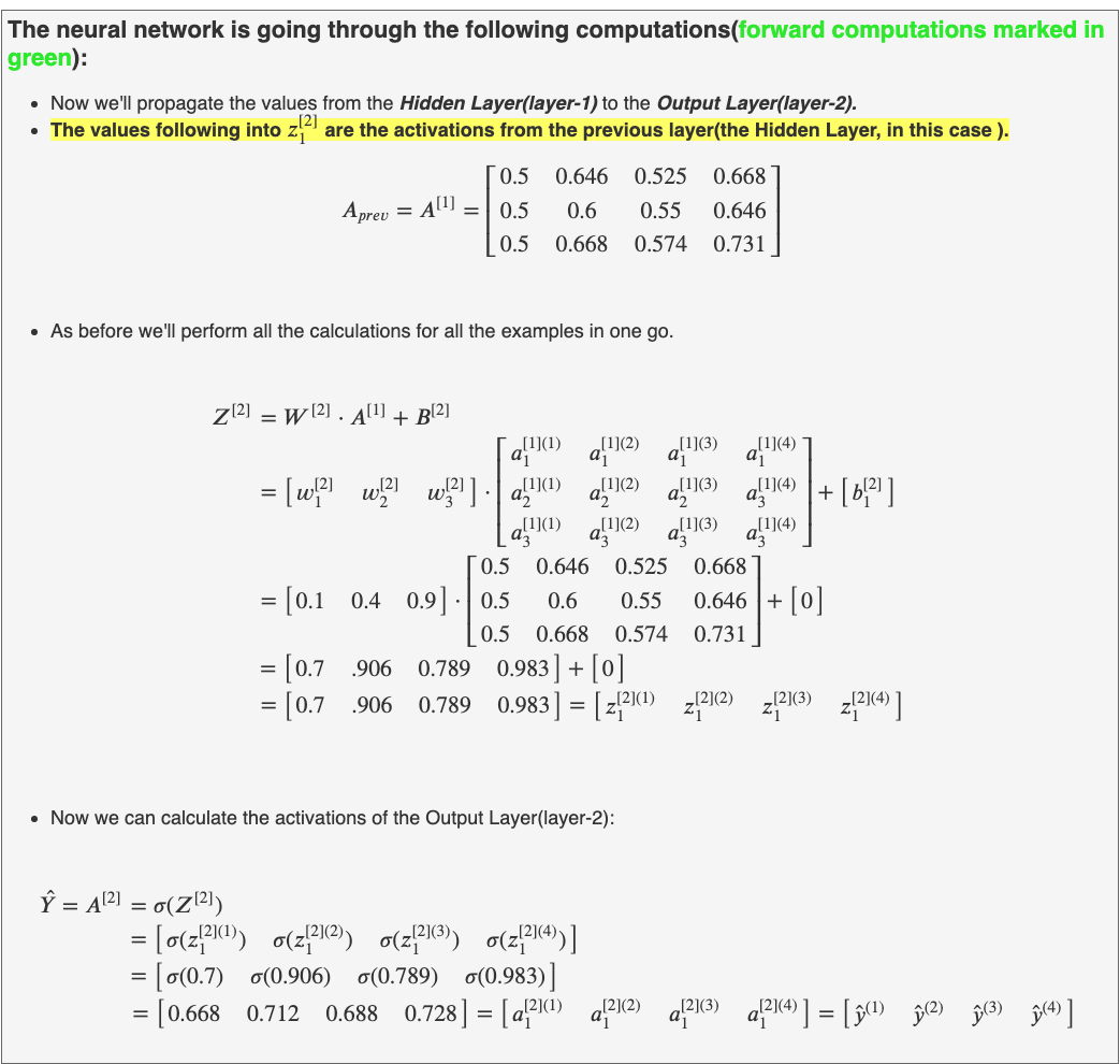
Now let’s perform a forward propagation:


We can now calculate the Cost:

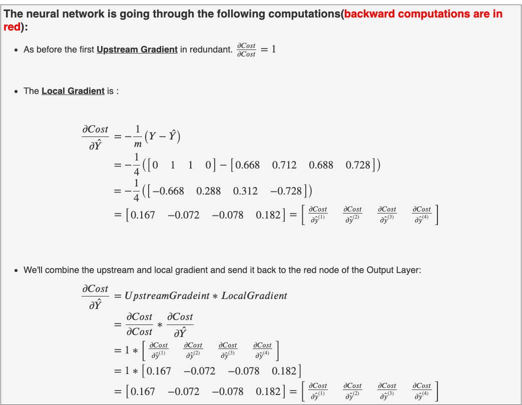
After the calculation of Cost, we can now do our backpropagation and improve the weights and biases.


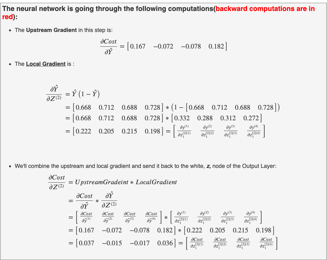

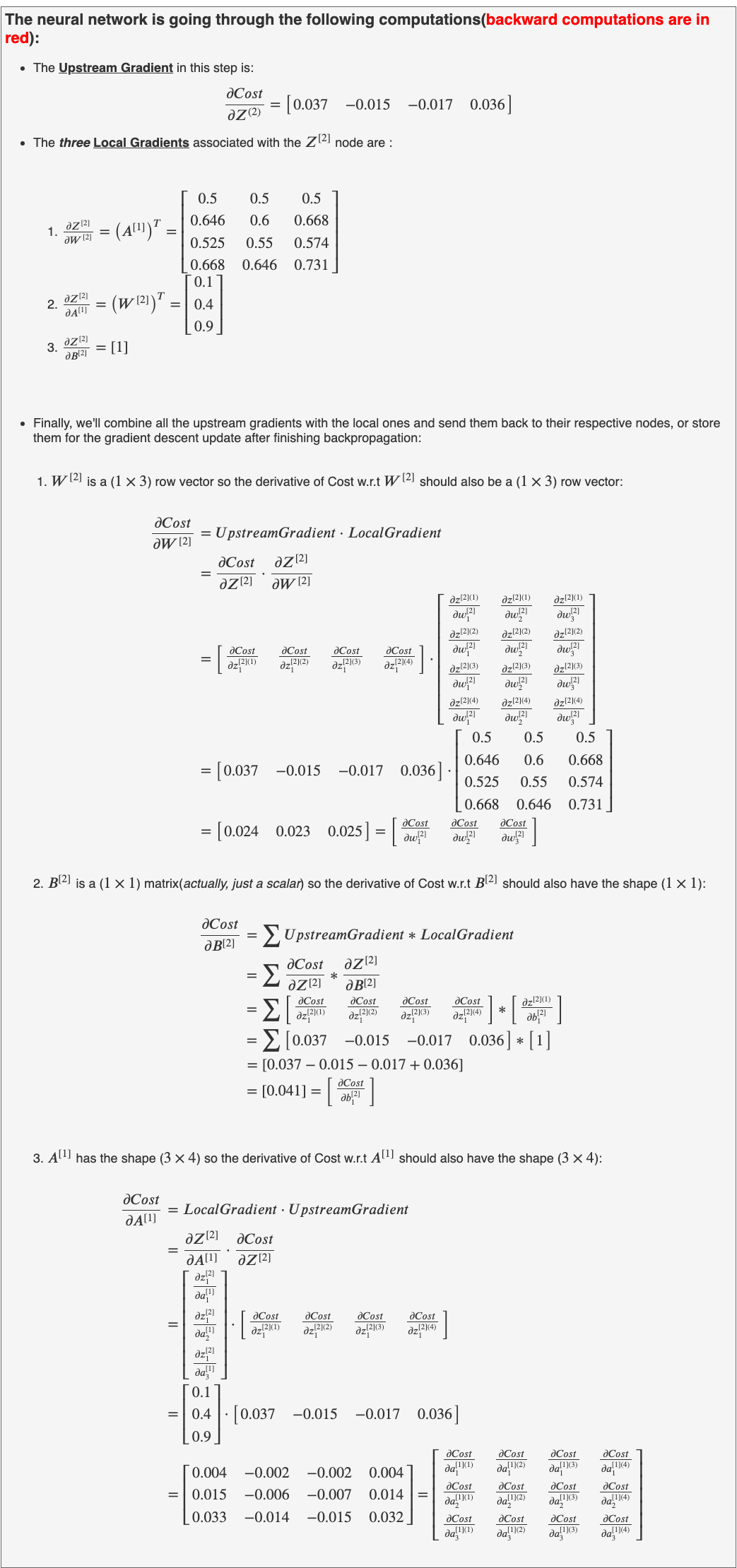

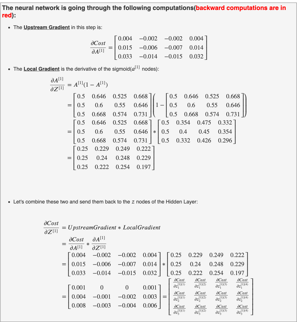

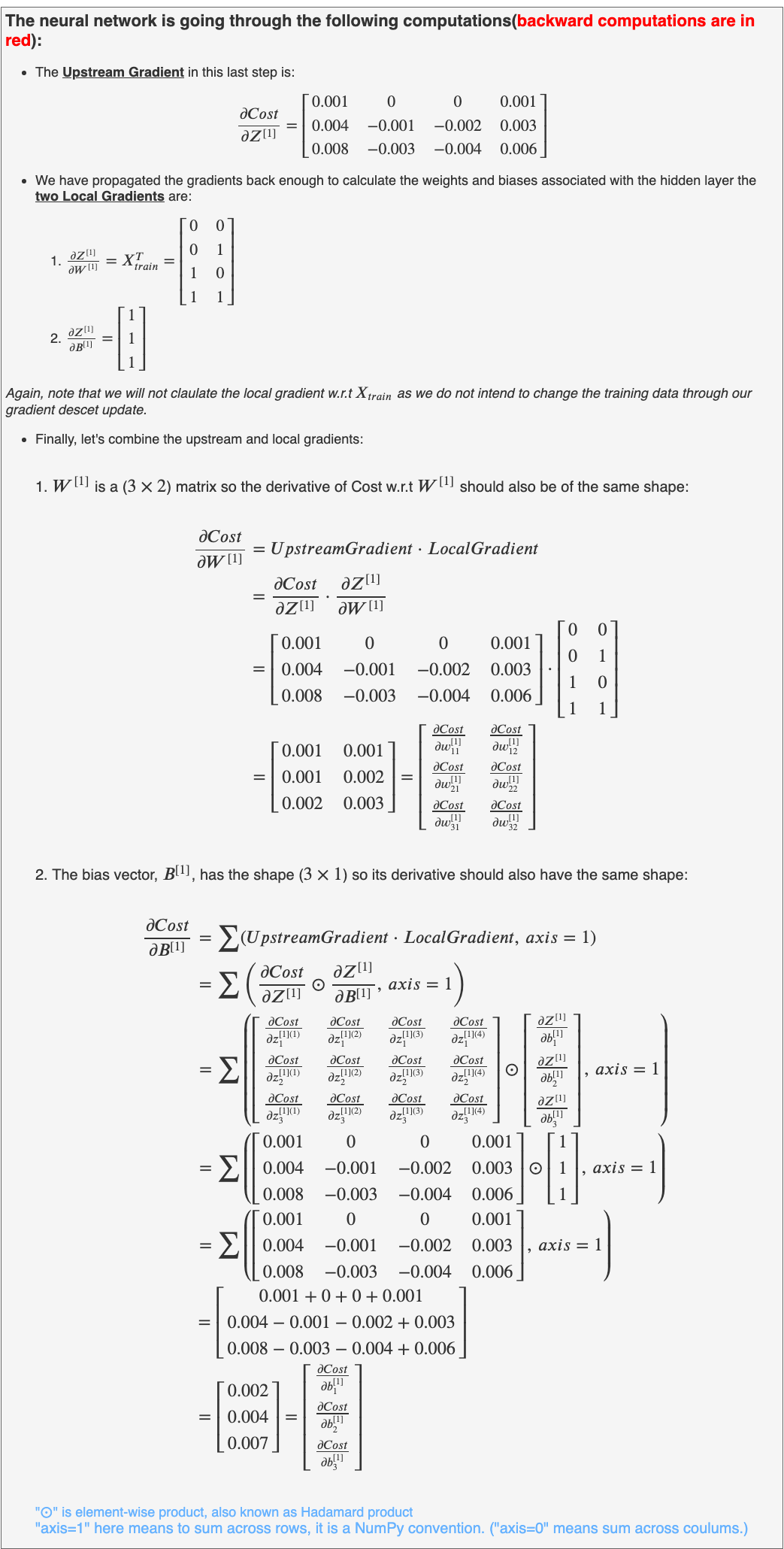
Whew! That was a lot, but it did a great deal to improve our understanding. Let’s perform the gradient descent update:

At this point, I would encourage all readers to perform one training iteration themselves. The resultant gradients should be approximately(rounded to 3 decimal places):

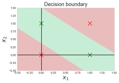
After 5000 epochs the Cost steadily decreases to about 0.0009 and we get the following Learning Curve and Decision Boundary:

Let’s also visualize where the decision of the neural network changes from 0(red) to 1(green):
This shows that the neural network has in fact learned where to fire-up(output 1) and where to lay dormant(output 0).
If we add another hidden layer with maybe 2 or 3 sigmoid neurons we can get an even more complex decision boundary that may fit our data even more tightly, but let’s leave that for the coding section.
Before we conclude this section I want to answer some remaining questions:
1- So, which one is better Feature Engineering or a Deep Neural Network?
Well, the answer depends on many factors. Generally, if we have a lot of training data we can just use a deep neural net to achieve acceptable accuracy, but if data is limited we may need to perform some feature engineering to extract more performance out of our neural network. As you saw in the feature engineering example above, to make good feature crosses one needs to have intimate knowledge of the dataset they are working with.
Feature engineering along with a deep neural network is a powerful combination.
2- How to count the number of layers in a Neural Network?
By convention, we don’t count layers without tunable weights and bias. Therefore, though the input layer is a separate “layer” we don’t count it when specifying the depth of a neural network.
So, our last example was a “2 layer neural network” (one hidden + output layer) and all the examples before it just a “1 layer neural network” (output layer, only).
3- Why use Activation Functions?
Activation functions are nonlinear functions and add nonlinearity to the neurons. The feature crosses are a result of stacking the activation functions in hidden layers. The combination of a bunch of activation functions thus results in a complex non-linear decision boundary. In this blog, we used the sigmoid/logistic activation function, but there are many other types of activation functions(ReLU being a popular choice for hidden layers) each providing a certain benefit. The choice of the activation function is also a hyper-parameter when creating neural networks.
Without activations functions to add nonlinearity, no matter how many linear functions we stack up the result of them will still be linear.Consider the following:
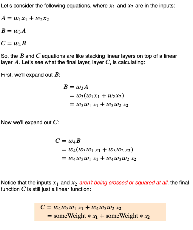
You may use any nonlinear function as an activation function. Some researchers have used even cos and sin functions. Preferably the activation function should be a continuous i.e. no breaks in the domain of the function.
4- Why Random Initialization of Weights?
This question is much easier to answer now. Note that if we had set all the weights in a layer to the same value than the gradient that passes through each node would be the same. In short, all the nodes in the layer would learn the same feature about the data. Setting the weights to random values helps in breaking the symmetry of weights so that each node in a layer has the opportunity to learn a unique aspect of the training data
There are many ways to set weights randomly in neural networks. For small neural networks, it is ok to set the weights to small random values. For larger networks, we tend to use “Xavier” or “He” initialization methods(will be in the coding section). Both these methods still set weights to random values but control their variance. For now, its suffice to say use these methods when the network does not seem to converge and the Cost becomes static or reduces very slowly when using the “plain” method of setting weights to small random values. Weight initialization is an active research area and will be a topic for a future “Nothing but Numpy” blog.
Biases can be randomly initialized, too. But in practice, it does not seem to have much of an effect on the performance of a neural network. Perhaps this is because the number of bias terms in a neural network is much fewer than the weights.
The type of neural network we created here is called a “fully-connected feedforward network” or simply a “feedforward network”.
This concludes Part Ⅰ.
Part Ⅱ: Coding a Modular Neural Network
The implementation in this part follows OOP principals.
Let’s first see the Linear Layer class. The constructor takes as arguments: the shape of the data coming in(input_shape), the number of neurons the layer outputs(n_out) and what type of random weight initialization need to be performed(ini_type=”plain”, default is “plain” which is just small random gaussian numbers).
The initialize_parameters is a helper function used to define weights and bias. We’ll look at it separately, later.
Linear Layer implements the following functions:
forward(A_prev): This function allows the linear layer to take in activations from the previous layer(the input data can be seen as activations from the input layer) and performs the linear operation on them.backward(upstream_grad): This function computes the derivative of Cost w.r.t weights, bias, and activations from the previous layer(dW,db&dA_prev, respectively)update_params(learning_rate=0.1): This function performs the gradient descent update on weights and bias using the derivatives computed in thebackwardfunction. The default learning rate(α) is 0.1
import numpy as np  # import numpy library
from util.paramInitializer import initialize_parameters  # import function to initialize weights and biases


class LinearLayer:
    """
        This Class implements all functions to be executed by a linear layer
        in a computational graph
        Args:
            input_shape: input shape of Data/Activations
            n_out: number of neurons in layer
            ini_type: initialization type for weight parameters, default is "plain"
                      Opitons are: plain, xavier and he
        Methods:
            forward(A_prev)
            backward(upstream_grad)
            update_params(learning_rate)
    """

    def __init__(self, input_shape, n_out, ini_type="plain"):
        """
        The constructor of the LinearLayer takes the following parameters
        Args:
            input_shape: input shape of Data/Activations
            n_out: number of neurons in layer
            ini_type: initialization type for weight parameters, default is "plain"
        """

        self.m = input_shape[1]  # number of examples in training data
        # `params` store weights and bias in a python dictionary
        self.params = initialize_parameters(input_shape[0], n_out, ini_type)  # initialize weights and bias
        self.Z = np.zeros((self.params['W'].shape[0], input_shape[1]))  # create space for resultant Z output

    def forward(self, A_prev):
        """
        This function performs the forwards propagation using activations from previous layer
        Args:
            A_prev:  Activations/Input Data coming into the layer from previous layer
        """

        self.A_prev = A_prev  # store the Activations/Training Data coming in
        self.Z = np.dot(self.params['W'], self.A_prev) + self.params['b']  # compute the linear function

    def backward(self, upstream_grad):
        """
        This function performs the back propagation using upstream gradients
        Args:
            upstream_grad: gradient coming in from the upper layer to couple with local gradient
        """

        # derivative of Cost w.r.t W
        self.dW = np.dot(upstream_grad, self.A_prev.T)

        # derivative of Cost w.r.t b, sum across rows
        self.db = np.sum(upstream_grad, axis=1, keepdims=True)

        # derivative of Cost w.r.t A_prev
        self.dA_prev = np.dot(self.params['W'].T, upstream_grad)

    def update_params(self, learning_rate=0.1):
        """
        This function performs the gradient descent update
        Args:
            learning_rate: learning rate hyper-param for gradient descent, default 0.1
        """

        self.params['W'] = self.params['W'] - learning_rate * self.dW  # update weights
        self.params['b'] = self.params['b'] - learning_rate * self.db  # update bias(es)
Fig 87. Linear Layer Class
Now let’s see the Sigmoid Layer class, its constructor takes in as an argument the shape of data coming in(input_shape) from a Linear Layer preceding it.
Sigmoid Layer implements the following functions:
forward(Z): This function allows the sigmoid layer to take in the linear computations(Z) from the previous layer and perform the sigmoid activation on them.backward(upstream_grad): This function computes the derivative of Cost w.r.t Z(dZ).
import numpy as np  # import numpy library

class SigmoidLayer:
    """
    This file implements activation layers
    inline with a computational graph model
    Args:
        shape: shape of input to the layer
    Methods:
        forward(Z)
        backward(upstream_grad)
    """

    def __init__(self, shape):
        """
        The consturctor of the sigmoid/logistic activation layer takes in the following arguments
        Args:
            shape: shape of input to the layer
        """
        self.A = np.zeros(shape)  # create space for the resultant activations

    def forward(self, Z):
        """
        This function performs the forwards propagation step through the activation function
        Args:
            Z: input from previous (linear) layer
        """
        self.A = 1 / (1 + np.exp(-Z))  # compute activations

    def backward(self, upstream_grad):
        """
        This function performs the  back propagation step through the activation function
        Local gradient => derivative of sigmoid => A*(1-A)
        Args:
            upstream_grad: gradient coming into this layer from the layer above
        """
        # couple upstream gradient with local gradient, the result will be sent back to the Linear layer
        self.dZ = upstream_grad * self.A*(1-self.A)
Fig 88. Sigmoid Activation Layer class
The initialize_parameters function is used only in the Linear Layer to set weights and biases. Using the size of input(n_in) and output(n_out) it defines the shape the weight matrix and bias vector need to be in. This helper function then returns both the weight(W) and bias(b) in a python dictionary to the respective Linear Layer.
def compute_cost(Y, Y_hat):
    """
    This function computes and returns the Cost and its derivative.
    The is function uses the Squared Error Cost function -> (1/2m)*sum(Y - Y_hat)^.2
    Args:
        Y: labels of data
        Y_hat: Predictions(activations) from a last layer, the output layer
    Returns:
        cost: The Squared Error Cost result
        dY_hat: gradient of Cost w.r.t the Y_hat
    """
    m = Y.shape[1]

    cost = (1 / (2 * m)) * np.sum(np.square(Y - Y_hat))
    cost = np.squeeze(cost)  # remove extraneous dimensions to give just a scalar

    dY_hat = -1 / m * (Y - Y_hat)  # derivative of the squared error cost function

    return cost, dY_hat
Fig 89. Helper function to set weights and bias
Finally, the Cost function compute_cost(Y, Y_hat) takes as argument the activations from the last layer(Y_hat) and the true labels(Y) and computes and returns the Squared Error Cost(cost) and its derivative(dY_hat).
def compute_cost(Y, Y_hat):
    """
    This function computes and returns the Cost and its derivative.
    The is function uses the Squared Error Cost function -> (1/2m)*sum(Y - Y_hat)^.2
    Args:
        Y: labels of data
        Y_hat: Predictions(activations) from a last layer, the output layer
    Returns:
        cost: The Squared Error Cost result
        dY_hat: gradient of Cost w.r.t the Y_hat
    """
    m = Y.shape[1]

    cost = (1 / (2 * m)) * np.sum(np.square(Y - Y_hat))
    cost = np.squeeze(cost)  # remove extraneous dimensions to give just a scalar

    dY_hat = -1 / m * (Y - Y_hat)  # derivative of the squared error cost function

    return cost, dY_hat
Fig 90. Function to compute Squared Error Cost and derivative.
At this point, you should open the 2_layer_toy_network_XOR Jupyter notebook from this repository in a separate window and go over this blog and the notebook side-by-side.
Now we are ready to create our neural network. Let’s use the architecture defined in Figure 77 for XOR data.
# define training constants
learning_rate = 1
number_of_epochs = 5000

np.random.seed(48) # set seed value so that the results are reproduceable
                  # (weights will now be initailzaed to the same pseudo-random numbers, each time)


# Our network architecture has the shape:
#                   (input)--> [Linear->Sigmoid] -> [Linear->Sigmoid] -->(output)

#------ LAYER-1 ----- define hidden layer that takes in training data
Z1 = LinearLayer(input_shape=X_train.shape, n_out=3, ini_type='xavier')
A1 = SigmoidLayer(Z1.Z.shape)

#------ LAYER-2 ----- define output layer that take is values from hidden layer
Z2= LinearLayer(input_shape=A1.A.shape, n_out=1, ini_type='xavier')
A2= SigmoidLayer(Z2.Z.shape)
Fig 91. Defining the layers and training parameters
Now we can start the main training loop:
costs = [] # initially empty list, this will store all the costs after a certian number of epochs

# Start training
for epoch in range(number_of_epochs):

    # ------------------------- forward-prop -------------------------
    Z1.forward(X_train)
    A1.forward(Z1.Z)

    Z2.forward(A1.A)
    A2.forward(Z2.Z)

    # ---------------------- Compute Cost ----------------------------
    cost, dA2 = compute_cost(Y=Y_train, Y_hat=A2.A)

    # print and store Costs every 100 iterations.
    if (epoch % 100) == 0:
        #print("Cost at epoch#" + str(epoch) + ": " + str(cost))
        print("Cost at epoch#{}: {}".format(epoch, cost))
        costs.append(cost)

    # ------------------------- back-prop ----------------------------
    A2.backward(dA2)
    Z2.backward(A2.dZ)

    A1.backward(Z2.dA_prev)
    Z1.backward(A1.dZ)

    # ----------------------- Update weights and bias ----------------
    Z2.update_params(learning_rate=learning_rate)
    Z1.update_params(learning_rate=learning_rate)
Fig 92. The training loop
Running the loop in the notebook we see that the Cost decreases to about 0.0009 after 4900 epochs
...
Cost at epoch#4600: 0.001018305488651183
Cost at epoch#4700: 0.000983783942124411
Cost at epoch#4800: 0.0009514180100050973
Cost at epoch#4900: 0.0009210166430616655
The Learning curve and Decision Boundaries look as follows:


The predictions our trained neural network produces are accurate.
The predicted outputs:
 [[ 0.  1.  1.  0.]]
The accuracy of the model is: 100.0%
Make sure to check out the other notebooks in the repository. We’ll be building upon the things we learned in this blog in future Nothing but NumPy blogs, therefore, it would behoove you to create the layer classes from memory as an exercise and try recreating the OR gate example from Part Ⅰ.
This concludes the blog. I hope you enjoyed.
For any questions feel free to reach out to me on twitter @RafayAK
This blog would not have been possible without following resources and people:
- Andrej Karpathy’s (@karpathy) Stanford course
- Christopher Olah’s (@ch402) blogs
- Andrew Trask’s (@iamtrask) blogs
- Andrew Ng (@AndrewYNg) and his Coursera courses on deep learningand machine learning
- Terence Parr (@the_antlr_guy) and Jeremy Howard (@jeremyphoward)(https://explained.ai/matrix-calculus/index.html)
- Ian Goodfellow (@goodfellow_ian) and his amazing book
- Finally, Hassan-uz-Zaman (@OKidAmnesiac) and Hassan Tauqeer for invaluable feedback.
Nothing but NumPy: Understanding & Creating Neural Networks with Computational Graphs from Scratch was originally published in Towards AI — Multidisciplinary Science Journal on Medium, where people are continuing the conversation by highlighting and responding to this story.
Published via Towards AI
Related posts


Comment (1)
Feedback ↓
Popular posts

 for 2021")


Updates

Recent Posts


Guillermo Correa
Hi Rafay!
I loved the post. I followed all the steps and made the suggested calculations.
Thank you very much! Greatly explained.
Only one coment. While trying to follow the Python part, I noticed that both figure 89 and figure 90 are the same, Function to compute Squared Error Cost and derivative.
I found Helper function to set weights and bias in Github.
Thank you again.
Guillermo Correa