Normal Equation in Linear Regression

Last Updated on June 25, 2020 by Editorial Team

Author(s): Saniya Parveez

Machine Learning

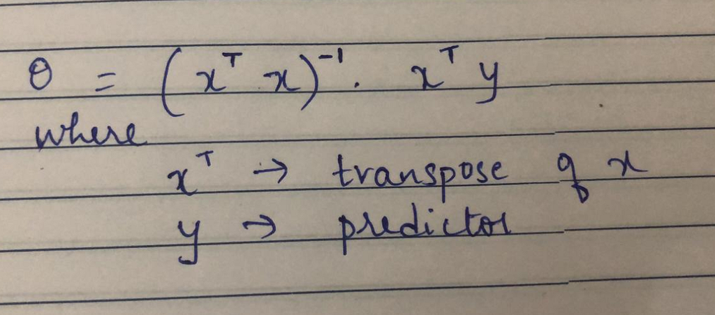
Gradient descent is a very popular and first-order iterative optimization algorithm for finding a local minimum over a differential function. Similarly, the Normal Equation is another way of doing minimization. It does minimization without restoring to an iterative algorithm. Normal Equation method minimizes J by explicitly taking its derivatives concerning theta j and setting them to zero.

Example:

Below is a data-set to predict house price:

House Features:

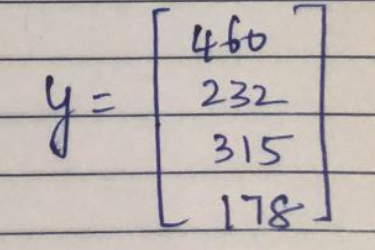
Predictor:

Calculation:

import numpy as np

x = np.array([[1, 2104, 5, 1, 45],
        [1, 1416, 3, 2, 40],
        [1, 1534, 3, 2, 30],
        [1, 852, 2, 1, 36]])

y = [460, 232, 315, 178]

x_transpose = x.transpose()

x_transpose_x = np.dot(x_transpose, x)

x_transpose_y = np.dot(x_transpose, y)

theta = np.dot(x_transpose_x_inverse, x_transpose_y)
theta

Gradient Descent Vs Normal Equation

Gradient Descent

• It requires to choose the value of Alpha.
• It requires many iterations.
• It works well when n (no. of data-set) is large.

Normal Equation

• It does not need to choose the value of Alpha.
• It doesn’t require iteration.
• It requires to calculate the inverse of transpose of x.
• It is slow if n (data-set) if very large.

Linear Regression with Normal Equation

Import libraries:

from numpy import genfromtxt
import numpy as np
from matplotlib import pyplot as plt
from sklearn.model_selection import train_test_split
from sklearn import linear_modl

Load the Portland data

data = genfromtxt('portland.csv', delimiter=',')

Feature extraction:

area = data[:, 0]

rooms =data[:, 1]

price = data[:, 2]

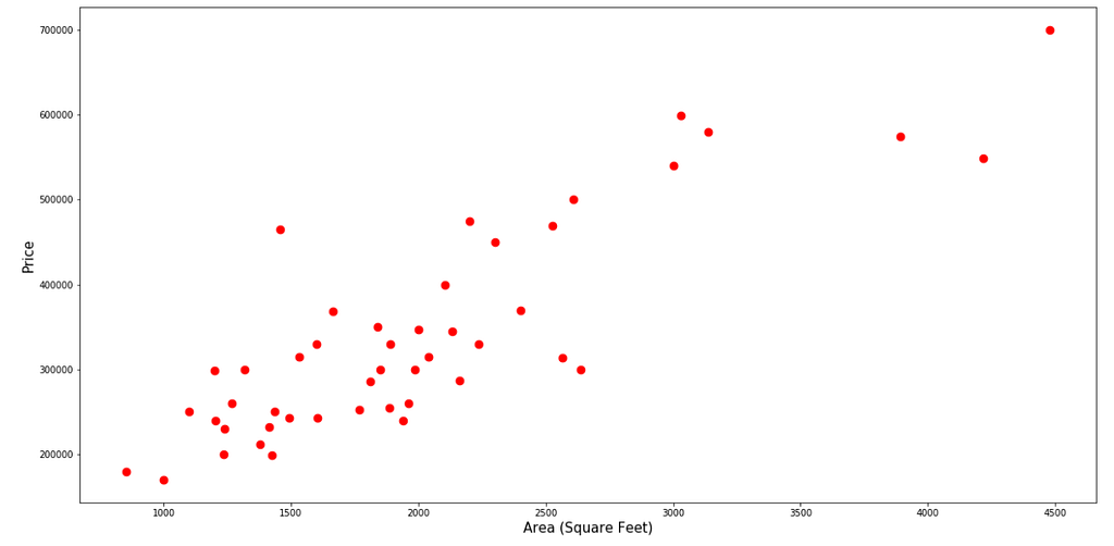
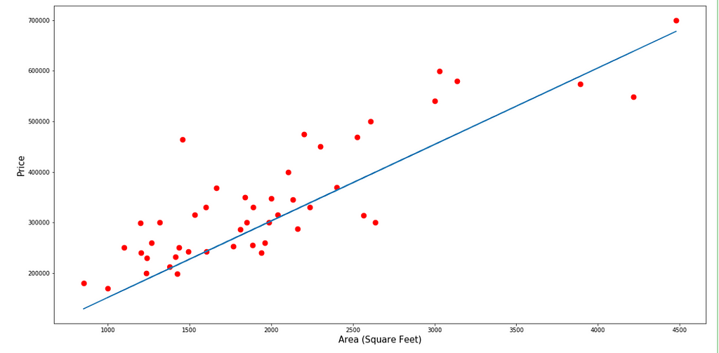
Visualize The Area against the Price:

def fitTheta(feature, theta):

return np.dot(theta, feature)

def visualiseFeature(feature, featureLabel, thetaVal=None):

fig = plt.figure(figsize=(20, 10))
    
    plt.rcParams.update({'font.size': 10})
    
    plt.xlabel(featureLabel, fontsize=15)
    
    plt.ylabel("Price", fontsize=15)
    
    plt.scatter(feature, price, color="red", s=75)
    
    if(thetaVal):
    
        thetaFit = fitTheta(feature, thetaVal)
        
        plt.plot(feature, thetaFit)

Visualize the Number of Rooms against the Price of the House:

visualiseFeature(rooms, "Number of Rooms")

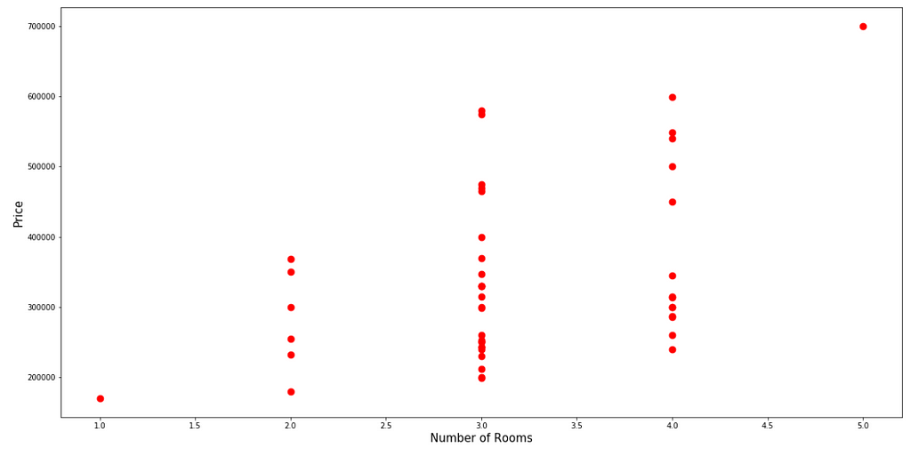
Here, the relationship between the Number of Rooms, and the Price of the House, appears to be Linear.

Define Feature Matrix, and Outcome/Target Vector:

X_data = data[:, 0:2] #Feature Matrix

y = data[:, 2] #Outcome Vector

Calculate Cost Function:

def getMSE(feature, thetaRange):
    costMatrix = np.repeat(price, thetaRange.shape[0]).reshape(price.shape[0], thetaRange.shape[0])
    
    costs = np.dot(np.asmatrix(feature).T, np.asmatrix(thetaRange)) - costMatrix
    
    MSE = (np.array((np.sum(costs, 0)))**2)/(2*price.shape[0])
    
    return np.array(MSE)[0]

Visualize Cost Function:

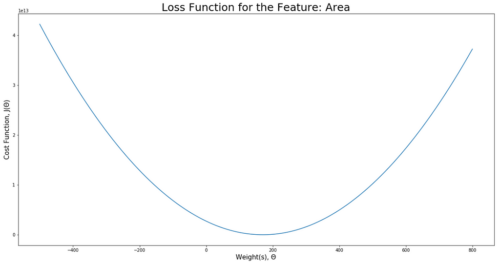
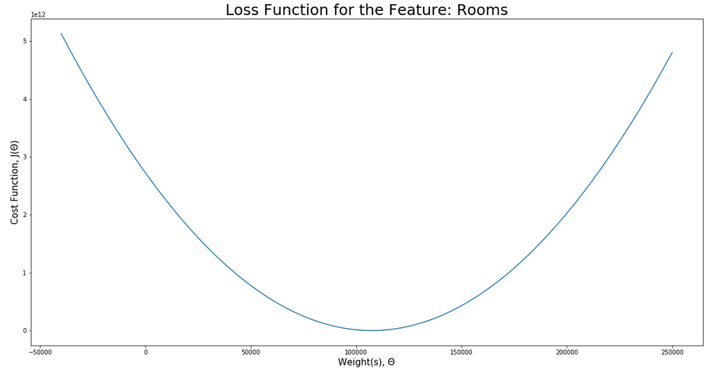
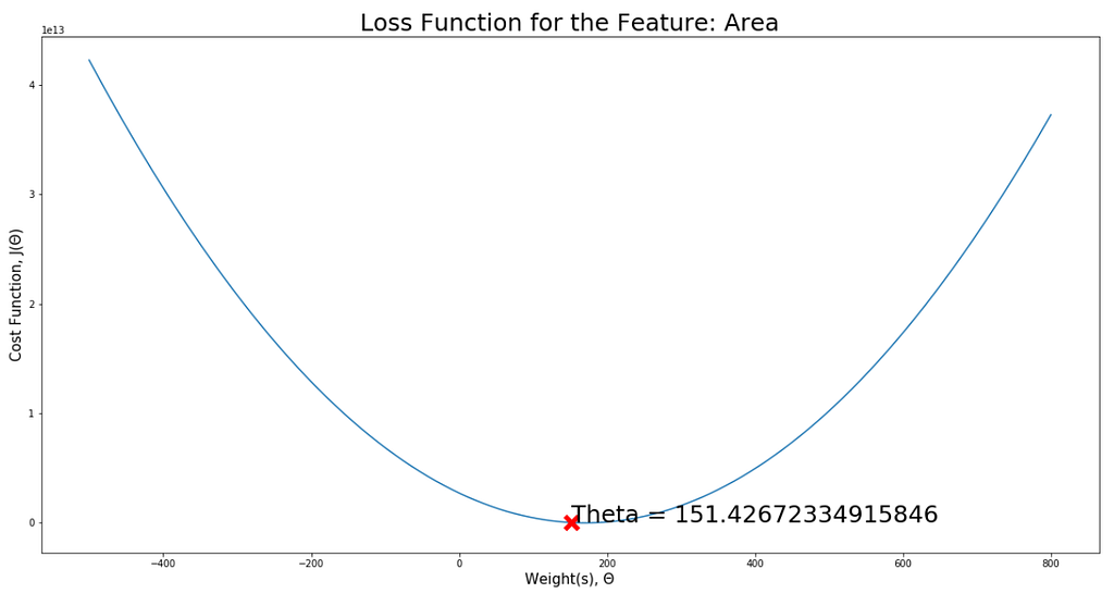
def visualiseLoss(feature, featureName, startInterval, endInterval, stepSize=0.5, thetaVal=None):
    thetaRange = np.arange(startInterval, endInterval, stepSize)
    
    Loss = getMSE(feature, thetaRange)
    
    fig = plt.figure(figsize=(20, 10))
    
    plt.title("Loss Function for the Feature: {}".format(featureName), fontsize=25)
    
    plt.ylabel("Cost Function, J(Θ)", fontsize=15)
    
    plt.xlabel("Weight(s), Θ", fontsize=15)
    
    plt.plot(thetaRange, Loss, zorder=1)
    
    if(thetaVal):
    
        thetaLoss = getMSE(feature, np.array(thetaVal).reshape(1, 1))
        
        plt.scatter(thetaVal, thetaLoss, marker="x", linewidth=5, color="red", s=200, zorder=2)
        
        plt.annotate("Theta = {}".format(thetaVal), (thetaVal, thetaLoss), fontsize=25)

visualiseLoss(area, "Area", -500, 800)

Add alt text

visualiseLoss(rooms, "Rooms", -40000, 250000)

Split Data

X_data = data[:, 0:2] #Feature Matrix

y = data[:, 2] #Outcome Vector

X = np.c_[np.ones(X_data.shape[0]), X_data]

X_train, X_test, y_train, y_test = train_test_split(X, y, test_size=0.2)

Normal Equation

firstTerm = np.linalg.inv(np.dot(X_train.T, X_train))

secondTerm = np.dot(X_train.T, y_train)

Theta = np.dot(firstTerm, secondTerm)

Visualize:

visualiseLoss(area, "Area", -500, 800, thetaVal=Theta[1])

visualiseFeature(area, "Area (Square Feet)", thetaVal=Theta[1])

Add alt text

Prediction using Normal Equation theta value

normal_predictions = np.dot(X_test, Theta)

normal_predictions

Add alt text

Prediction using Linear Regression

reg = linear_model.LinearRegression()

reg.fit(X_train, y_train)

sk_predictions = reg.predict(X_test)

sk_predictions

Add alt text

Here, the predictions from the Normal Equation and Linear Equation are the same.

Normal Equation Non-Invertibility

A squared matrix that does not have an inverse a matrix is singular if and only if it is determined is zero.

Example:

import numpy as np

A = [[2, 6],

[1, 3]]

The inverse of Matrix:

inverse_A = np.linalg.inv(A)

inverse_A

Error from Numpy:

Add alt text

Problem due to Non-Invertibility:

• Redundant features
• Too many features

How to solve if there are too many features?

• Delete some features of use Regularization

Conclusion

Gradient Descent gives one way to minimizing J. Normal Equation is another way of doing minimization. It does minimization without restoring to an iterative algorithm. But, Normal Equation is very slow if the data-set size is very large

---

Normal Equation in Linear Regression was originally published in Towards AI — Multidisciplinary Science Journal on Medium, where people are continuing the conversation by highlighting and responding to this story.

Published via Towards AI