Stock Price Prediction Model for Netflix

Last Updated on May 24, 2022 by Editorial Team

A Comparative Study of Linear Regression, K-Nearest Neighbor (KNN) and Support Vector Machine (SVM)

Author(s): Vivek Chaudhary

The objective of this article is to design a stock prediction linear model to predict the closing price of Netflix. This will be a comparative study of various machine learning models such as linear regression, K-nearest neighbor, and support vector machines.

Before designing the model I was going through some of the investment-related blogs and articles on the internet to get a better understanding of the matter and I found out some key indicators that determine the opening and closing price of a stock. Therefore, this tutorial on the training of the model will not be limited to a single feature instead this will be a multi-feature trained model.

Stock Market Basic Influencing Factor

As a data scientist or an ml pro it eases out our work when we have a business or functional clarity on what we are trying to build, so I thought I must share some business insight as well, however, I am not a stock market pro but I thought it will build an understanding. so basically the closing price is the last price a buyer paid for that particular stock during business hours and the opening price is the price of the first transaction of that stock, and it is a very common phenomenon in stock trading that an opening price can be different from the closing price, the reason being the fluctuation between demand and supply that determines the attractiveness of a stock. this phenomenon is termed as AHT (after-hours trading) which plays a pivotal role in shifting the opening price of a stock. there are other factors as well as I am not an expert on such matters so I am not going to dig deep into it. this small snippet of information was to give a basic insight into the real-world problem.
so without wasting a further ado lets jump to the solution “coding”

1. Import prerequisites:

import pandas as pd
from sklearn.linear_model import LinearRegression
from sklearn.model_selection import train_test_split
import matplotlib.pyplot as plt
import numpy as np
import pandas_datareader as web

pandas_datareader library allows us to connect to the website and extract data directly from internet sources in our case we are extracting data from Yahoo Finance API.

2. Read and Display

df = web.DataReader(‘NFLX’, data_source=’yahoo’, start=’2012–01–01', end=’2020–04–28')
df.tail(10)

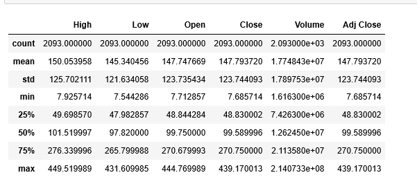
df.reset_index(inplace=True)
df.describe()

3. Check for Correlation

Before we check for correlation lets understand what exactly it is?

Correlation is a measure of association or dependency between two features i.e. how much Y will vary with a variation in X. The correlation method that we will use is the Pearson Correlation.

Pearson Correlation Coefficient is the most popular way to measure correlation, the range of values varies from -1 to 1. In mathematics/physics terms it can be understood as if two features are positively correlated then they are directly proportional and if they share negative correlation then they are inversely proportional.

corr = df.corr(method=’pearson’)
corr

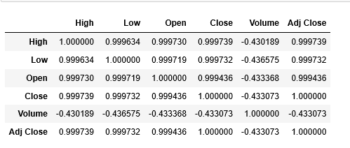
Not all text is understandable, lets visualize the correlation coefficient.

import seaborn as sb
sb.heatmap(corr,xticklabels=corr.columns, yticklabels=corr.columns,
 cmap='RdBu_r', annot=True, linewidth=0.5)

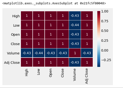
The Dark Maroon zone is not Maroon5, haha joking, but it denotes the highly correlated features.

4. Visualize the Dependent variable with Independent Features

#prepare dataset to work with 
nflx_df=df[[‘Date’,’High’,’Open’,’Low’,’Close’]]
nflx_df.head(10)

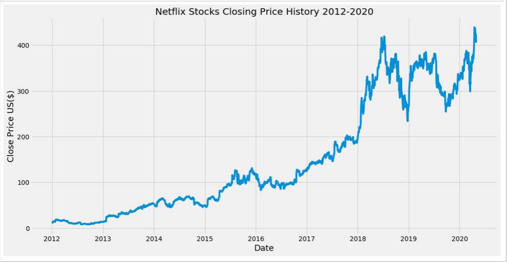
plt.figure(figsize=(16,8))
plt.title('Netflix Stocks Closing Price History 2012-2020')
plt.plot(nflx_df['Date'],nflx_df['Close'])
plt.xlabel('Date',fontsize=18)
plt.ylabel('Close Price US($)',fontsize=18)
plt.style.use('fivethirtyeight')
plt.show()

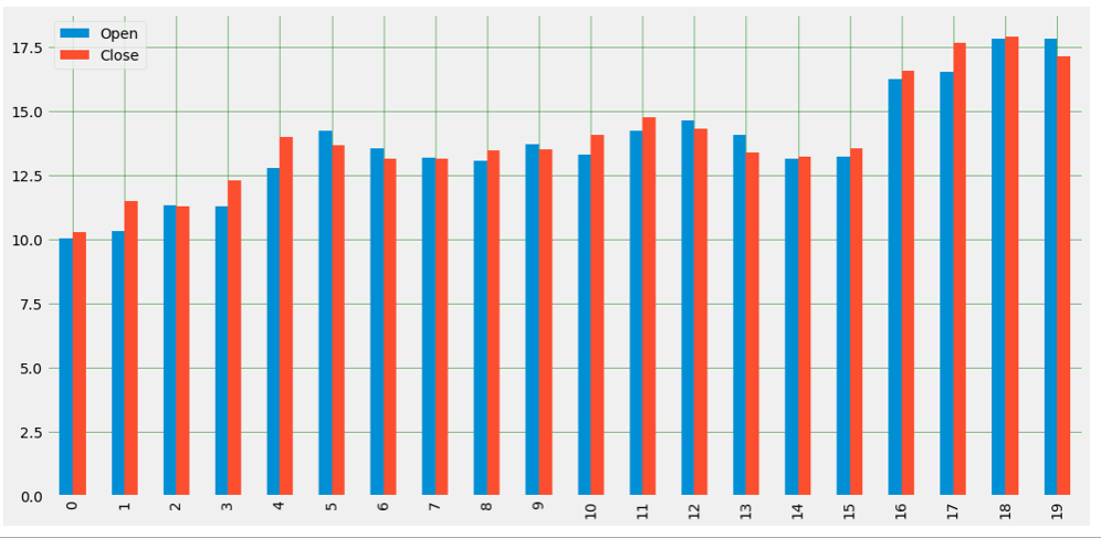
#Plot Open vs Close
nflx_df[['Open','Close']].head(20).plot(kind='bar',figsize=(16,8))
plt.grid(which='major', linestyle='-', linewidth='0.5', color='green')
plt.grid(which='minor', linestyle=':', linewidth='0.5', color='black')
plt.show()

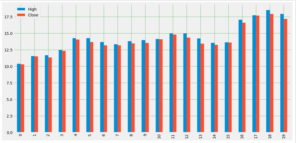
#Plot High vs Close
nflx_df[['High','Close']].head(20).plot(kind='bar',figsize=(16,8))
plt.grid(which='major', linestyle='-', linewidth='0.5', color='green')
plt.grid(which='minor', linestyle=':', linewidth='0.5', color='black')
plt.show()

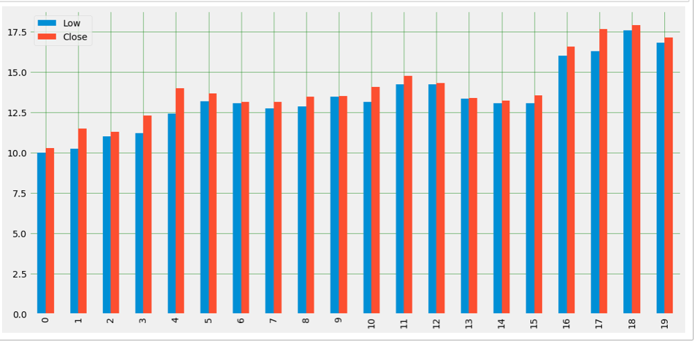
#Plot Low vs Close
nflx_df[[‘Low’,’Close’]].head(20).plot(kind=’bar’,figsize=(16,8))
plt.grid(which=’major’, linestyle=’-’, linewidth=’0.5', color=’green’)
plt.grid(which=’minor’, linestyle=’:’, linewidth=’0.5', color=’black’)
plt.show()

5. Model Training and Testing

#Date format is DateTime and it will throw error while training so I have created seperate month, year and date entities

nflx_df[‘Year’]=df[‘Date’].dt.year
nflx_df[‘Month’]=df[‘Date’].dt.month
nflx_df[‘Day’]=df[‘Date’].dt.day

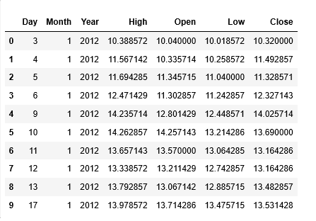
Create the final dataset for Model training

nfx_df=nflx_df[[‘Day’,’Month’,’Year’,’High’,’Open’,’Low’,’Close’]]
nfx_df.head(10)

#separate Independent and dependent variable
X = nfx_df.iloc[:,nfx_df.columns !=’Close’]
Y= nfx_df.iloc[:, 5]

print(X.shape) #output: (2093, 6)
print(Y.shape) #output: (2093,)

Splitting the dataset into train and test

from sklearn.model_selection import train_test_split
x_train,x_test,y_train,y_test= train_test_split(X,Y,test_size=.25)

print(x_train.shape) #output: (1569, 6)
print(x_test.shape) #output: (524, 6) 
print(y_train.shape) #output: (1569,)
print(y_test.shape) #output: (524,)
#y_test to be evaluated with y_pred for Diff models

Model 1: Linear Regression

Linear Regression Model Training and Testing

lr_model=LinearRegression()
lr_model.fit(x_train,y_train)

y_pred=lr_model.predict(x_test)

Linear Model Cross-Validation

What is exactly Cross-Validation?

Basically Cross Validation is a technique using which Model is evaluated on the dataset on which it is not trained i.e. it can be a test data or can be another set as per availability or feasibility.

from sklearn import model_selection
from sklearn.model_selection import KFold
kfold = model_selection.KFold(n_splits=20, random_state=100)
results_kfold = model_selection.cross_val_score(lr_model, x_test, y_test.astype('int'), cv=kfold)
print("Accuracy: ", results_kfold.mean()*100)

#output: Accuracy: 99.999366595175

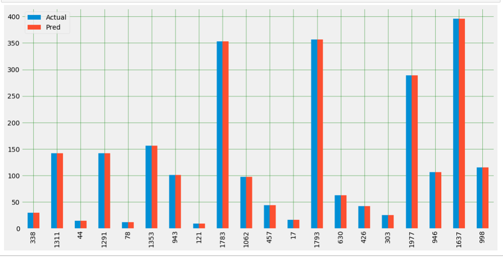
Plot Actual vs Predicted Value

plot_df=pd.DataFrame({‘Actual’:y_test,’Pred’:y_pred})
plot_df.head(20).plot(kind='bar',figsize=(16,8))
plt.grid(which='major', linestyle='-', linewidth='0.5', color='green')
plt.grid(which='minor', linestyle=':', linewidth='0.5', color='black')
plt.show()

Model 2: KNN K-nearest neighbor Regression Model

KNN Model Training and Testing

from sklearn.neighbors import KNeighborsRegressor
knn_regressor=KNeighborsRegressor(n_neighbors = 5)
knn_model=knn_regressor.fit(x_train,y_train)
y_knn_pred=knn_model.predict(x_test)

KNN Cross-Validation

knn_kfold = model_selection.KFold(n_splits=20, random_state=100)
results_kfold = model_selection.cross_val_score(knn_model, x_test, y_test.astype(‘int’), cv=knn_kfold)
print(“Accuracy: “, results_kfold.mean()*100)

#output: Accuracy: 99.93813335235933

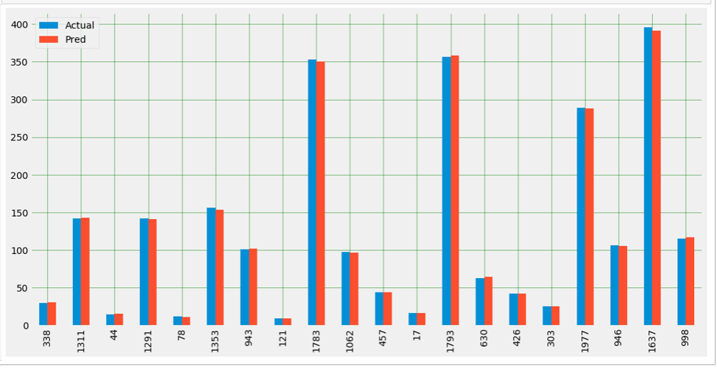
Plot Actual vs Predicted

plot_knn_df=pd.DataFrame({‘Actual’:y_test,’Pred’:y_knn_pred})
plot_knn_df.head(20).plot(kind=’bar’,figsize=(16,8))
plt.grid(which=’major’, linestyle=’-’, linewidth=’0.5', color=’green’)
plt.grid(which=’minor’, linestyle=’:’, linewidth=’0.5', color=’black’)
plt.show()

Model 3: SVM Support Vector Machine Regression Model

SVM Model Training and Testing

from sklearn.svm import SVR
svm_regressor = SVR(kernel=’linear’)
svm_model=svm_regressor.fit(x_train,y_train)
y_svm_pred=svm_model.predict(x_test)

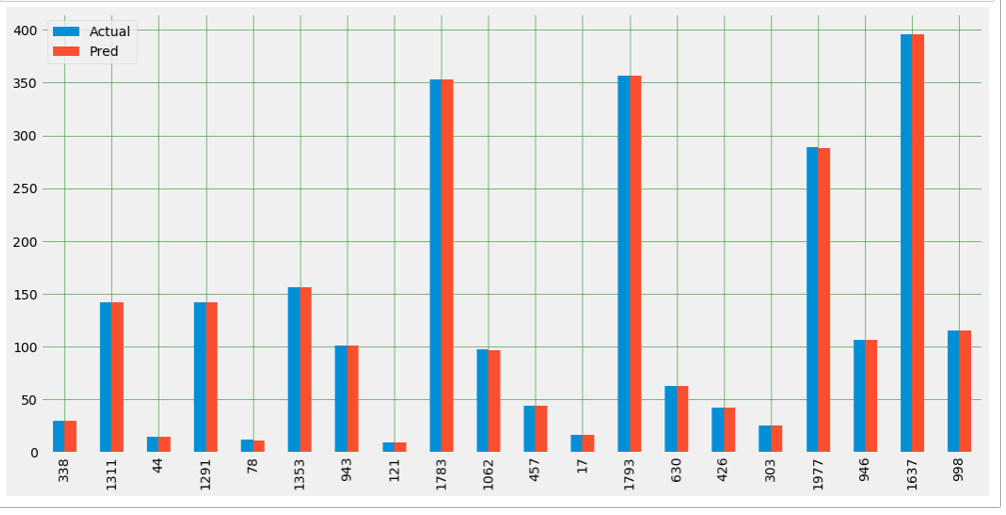
Plot Actual vs Predicted

plot_svm_df=pd.DataFrame({‘Actual’:y_test,’Pred’:y_svm_pred})
plot_svm_df.head(20).plot(kind=’bar’,figsize=(16,8))
plt.grid(which=’major’, linestyle=’-’, linewidth=’0.5', color=’green’)
plt.grid(which=’minor’, linestyle=’:’, linewidth=’0.5', color=’black’)
plt.show()

RMSE (Root Mean Square Error)

Root Mean Square Error is the Standard Deviation of residuals, which are a measure of how far data points are from the regression. Or in simple terms how concentrated the data points are around the best fit line.

from sklearn.metrics import mean_squared_error , r2_score
import math

lr_mse=math.sqrt(mean_squared_error(y_test,y_pred))
print(‘Linear Model Root mean square error’,lr_mse)

knn_mse=math.sqrt(mean_squared_error(y_test,y_knn_pred))
print(‘KNN Model Root mean square error’,mse)

svm_mse=math.sqrt(mean_squared_error(y_test,y_svm_pred))
print(‘SVM Model Root mean square error SVM’,svm_mse)

#outputs as below:
Linear Model Root mean square error 1.7539775065782694e-14 
KNN Model Root mean square error 1.7539775065782694e-14 
SVM Model Root mean square error SVM 0.0696764093622963

R2 or r-squared error

R2 or r2 score varies between 0 to 100%.

Mathematical Formula for r2 score :(y_test[i] — y_pred[i]) **2

print(‘Linear R2: ‘, r2_score(y_test, y_pred))
print(‘KNN R2: ‘, r2_score(y_test, y_knn_pred))
print(‘SVM R2: ‘, r2_score(y_test, y_svm_pred))

#output as below:
Linear R2: 1.0 
KNN R2: 0.9997974105145412 
SVM R2: 0.9999996581785765

For basic mathematical understanding on RMSE and R2 error refer my blog: https://www.geeksforgeeks.org/ml-mathematical-explanation-of-rmse-and-r-squared-error/

Our Model looks very much good with phenomenal stats.

Summary:

· Use of prerequisite libraries

· Data extraction from the web using pandas_datareader

· Basic Stocks understanding

· Model training and testing

· ML algorithms such as Linear Regression, K-nearest neighbor and Support Vector Machines

· Kfold Cross-Validation of Models

· Python seaborn library to visualize correlation heatmap

· Pearson correlation

· Feature plotting against dependent output using Matplotlib.

· Plotting of Actual value with the Predicted value.

· Root Mean Square Error (RMSE).

· R-squared error

Thanks to all for reading my blog and If you like my content and explanation please follow me on medium and share your feedback, which will always help all of us to enhance our knowledge.

Thanks for reading!

Vivek Chaudhary

---

Stock Price Prediction Model for Netflix was originally published in Towards AI — Multidisciplinary Science Journal on Medium, where people are continuing the conversation by highlighting and responding to this story.