Linear Regression from Scratch

Author(s): Nunzio Logallo

Originally published on Towards AI.

If you started to learn data science or machine learning, you have also heard about linear regression, but what is it and when should we use it?

Linear Regression is a statistical model and a supervised algorithm; we use it to predict linear value, this means that we try to fit a line along with our data and predict the independent variable from it. To understand better linear regression, let us start from its equation.

Where y is the predicted value, x the independent variable, m is the slope, and b is the y-intercept, the point where the line intersects the y-axis. The slope indicates the inclination of the line, where 0 indicates a horizontal line, but generally, the equation is:

After this short theoretical introduction, let us explain how to train and test our first linear regression model. We will use a linear regression model to predict salary based on the years of experience. First of all, we have to be sure that what we are trying to predict is a linear value; a method to understand if a linear regression model can fit our data is to visualize them, let us look at a sample dataset plot:

salary = df["Salary"]
years_experience = df["YearsExperience"]#generating the scatter plot
plt.figure(figsize=(7, 5))
plt.scatter(years_experience, salary)
plt.xlabel("Years of Experience")
plt.ylabel("Salary")

The result of the code above will be something like this:

As you can see, the values plotted in this scatter plot describe a line. Then we can say that a linear regression model can fit this data. Now let us train a linear regression model with Sklearn:

#train test split
X_train, X_test, y_train, y_test = train_test_split(X, y, test_size=0.3, random_state=0)#training
lr = LinearRegression().fit(X_train,y_train)

Congratulations, you have trained a linear regression model! Now, we have to take a look at the results. Let us have a first look at the intersect and slope of the line.

print("Intercept = ", lr.intercept_)
print("Slope = ", lr.coef_)#output
Intercept = 26777.391341197625
Slope = [9360.26128619]

Let us test our model predicting some values from the test set.

y_pred = lr.predict(X_test)df = pd.DataFrame({"Actual": y_test, "Predicted": y_pred})
df

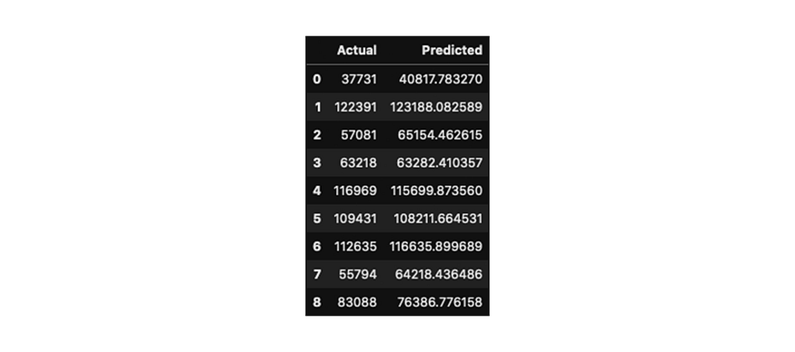
As you can see from the results, the predicted values are near to the actual values, but they are not the same, that is because the line does not fit perfectly each value, let us have a look at the line itself.

#generating the scatter plot
plt.scatter(X_test, y_test)
plt.plot(X_test, y_pred, color="red", linewidth=2)
plt.xlabel("Years of Experience")
plt.ylabel("Salary")

Blue dots indicate the actual values on the test set, while the red line is the predictions based on the trained data. As you can see, there is a distance between actual values and prediction line, this distance is called residual, and we can calculate it: residual = actual value — predicted value.

Evaluation

There are different metrics to evaluate our regression model: let us see the three most important:

• Mean Squared Error (MSE) is the average squared difference between the estimated value and the actual value. This is the most popular metric because it focuses on larger errors due to the squared term that exponentially increases larger errors in comparison to smaller ones.

• Mean Absolute Error(MAE) is the average difference between the estimated value and the actual value. This is the most straightforward metric to understand since it is just an average error.

• Root Mean Squared Error (RMSE) is the square root of the average difference between the estimated value and the actual value; basically, the square root of the mean squared error.

• R-squared is a popular metric, not an error, and it represents how close the data are to the fitted regression line. The higher the score, the better the model fits your data. The best possible score is 1.0, but it can also be negative for a bad model.

In the formulas above, n indicates the number of predictions, y the vector of actual values, and yi the vector of predicted values.

The model we just trained is also called Simple Linear Regression because there is only one independent variable.

Multiple Linear Regression

In Multiple Linear Regression, we have more than one independent variable, and this means that we can check the effects that more features have on the dependent variable. Multiple Linear Regression is instrumental when you are examining your dataset because you can compare different features and check how different is their impact on the dependent variable so that you can choose only the best ones. Let us have a look to its formula:

In the formula above, b is the y-intercept, m is the coefficient of each feature, while x represents each feature; we will better understand this with an example dataset.

The dataset we will use to explain Multiple Linear Regression better is the fuel consumption dataset, we will create a multiple linear regression model to see the impact of multiple features (engine size, cylinders, and fuel consumption) on the dependent variable(CO2 emissions). Let us see a first scatter plot representing the relation between engine size and CO2 emissions.

#generating the scatter plot
plt.figure(figsize=(7, 5))
plt.scatter(df.ENGINESIZE, df.CO2EMISSIONS, color='blue')
plt.xlabel("Engine size")
plt.ylabel("CO2 Emissions")

The other two representing the relations that the other two features we are examining have with CO2 emissions are pretty different and less linear than the first one:

Let us train a Multiple Regression model with these three features:

#train test split randomly with numpy
msk = np.random.rand(len(df)) < 0.8
train = df[msk]
test = df[~msk]
X_train = np.asanyarray(train[['ENGINESIZE','CYLINDERS','FUELCONSUMPTION_COMB']])
y_train = np.asanyarray(train[['CO2EMISSIONS']])#training
lr.fit (X_train, y_train)

As we saw from the formula, there is the y-intercept, and there are multiple coefficients, one for each feature.

print ("Intercept: ", lr.intercept_)
print ("Coefficients: ", lr.coef_)#output
Intercept: [67.3968258]
Coefficients: [[10.23919289 7.99343458 9.31617168]]

Now that we trained our model to let us evaluate it, predicting some values in the test set.

y_pred= lr.predict(test[['ENGINESIZE','CYLINDERS','FUELCONSUMPTION_COMB']])
X_test = np.asanyarray(test[['ENGINESIZE','CYLINDERS','FUELCONSUMPTION_COMB']])
y_test = np.asanyarray(test[['CO2EMISSIONS']])

Now, let us see its score numerically, calculating the MSE, MAE, RMSE, and the R-Squared score.

print("Mean Squared Error:", metrics.mean_squared_error(y_test, y_pred)) 
print("Mean Absolute Error: ", metrics.mean_absolute_error(y_test, y_pred))
print("Root Mean Squared Error: ", np.sqrt(metrics.mean_squared_error(y_test, y_pred)))
print("R-Squared Score: ", metrics.r2_score(y_test, y_pred))#output
Mean Squared Error: 513.8862607223467
Mean Absolute Error: 16.718115229014394
Root Mean Squared Error: 22.66905954649082
R-Squared Score: 0.8789478910480176

Moreover, we are done! We learned how Linear Regression works, we trained and evaluated a Simple Linear Regression Model and a Multiple Linear Regression Model. If you want to learn more about Linear Regression, you can visit my GitHub, where you can see my notebook about it.

Thanks for reading.

Join thousands of data leaders on the AI newsletter. Join over 80,000 subscribers and keep up to date with the latest developments in AI. From research to projects and ideas. If you are building an AI startup, an AI-related product, or a service, we invite you to consider becoming a sponsor.

Published via Towards AI