What? How? Why? — In the World of Data Science!

Author(s): Deepak Sekar

Originally published on Towards AI.

In this article, we will see the three things that matter the most in the Data Science Process

1. What — What is the Business requirement? What are the data sources and features? What is the outcome?
2. How — How to build a model? How good is the model? How long it is going to take?
3. Why — Why did the model predict such an outcome?

We will take a simple use-case to understand why?

Note: Basic Python, Data Science knowledge expected.

What?

Company X is serving a large customer base and is recently facing an increased churn rate (the rate at which customers are moving out). So the CIO has asked the Data Science Lead to create a churn prediction model and create a risk profile for the existing customers.

The target is just one variable that says whether a customer is “At-risk” or “Not at risk”

The Data Science Lead then interacts with the data owners/ business folks to understand the spread of the data and sources. Company X has all the relevant data in Oracle’s Autonomous Database.

How?

The Data Science Lead comes up with a plan!

• *Autonomous Database — https://www.oracle.com/au/database/autonomous-database.html
• *Oracle Cloud Infrastructure Data Science Platform — https://www.oracle.com/data-science/cloud-infrastructure-data-science-product.html

1. Setting up the Data Science Environment in Oracle Cloud in 2 clicks!

a. Spin up a Data Science instance and create a project

b. Create a Jupyterlab notebook session and choose the required Infrastructure.

(I am going to use an Intel Xeon — 2 OCPU VM with 100 GB block storage within a private subnet (Each OCPU includes the complete processor core along with the hyperthreading unit)

And there it is — ready to use right away!

2. Connecting to the Oracle Autonomous Data Warehouse (ADW) in the Cloud within the JupyterLab Notebook (You will need the ADW database wallet stored locally for authentication)

%env TNS_ADMIN=/home/datascience/block_storage/ADWWallet
%env ADW_SID=<>
%env ADW_USER=<>
%env ADW_PASSWORD=<>
!echo exit U+007C sqlplus $ADW_USER/$ADW_PASSWORD@$ADW_SID

3. Loading the data from a table in ADW

With Dask you can profile the compute graph and also visualize the profiler output. Bokeh extension for JupyterLab lets you render the visualization within your notebook. ADS provides you a decorator that leverages Dask profiler to help you visualize the CPU and memory utilization of supported operations.

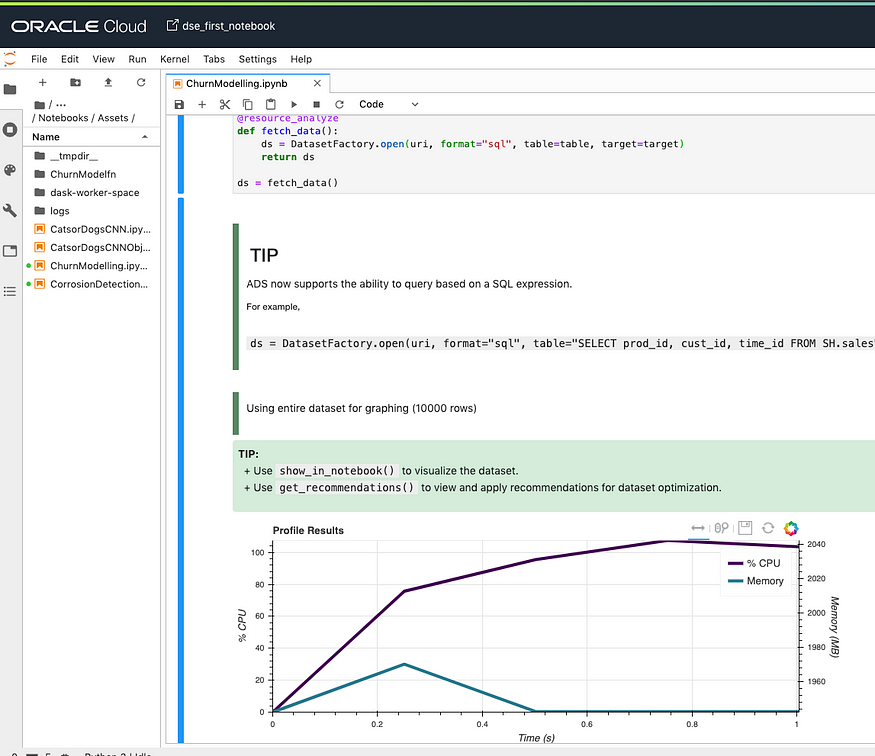
from ads.common.analyzer import resource_analyze
from ads.dataset.factory import DatasetFactory@resource_analyze
def fetch_data():
ds = DatasetFactory.open(uri, format="sql", table=table, target=target)
return dsds = fetch_data()

One cool thing is that you can specify the target variable while the data is being loaded!

%load_ext autoreload
%autoreload 2
import warnings
warnings.filterwarnings("ignore")
import pandas as pd
import logging
import oslogging.basicConfig(format='%(levelname)s:%(message)s', level=logging.INFO)from ads.dataset.factory import DatasetFactoryuri=f'oracle+cx_oracle://{os.environ["ADW_USER"]}:{os.environ["ADW_PASSWORD"]}@{os.environ["ADW_SID"]}'
table = "<>"# Optional. Leave it as-is if you don't want to specify a target value: 
target = "<>"
if target != "":
 ds = DatasetFactory.open(uri, format="sql", table=table, target=target)
else: 
 ds = DatasetFactory.open(uri, format="sql", table=table)

4. Understanding the data

Using one method “show_in_notebook()” from DatasetFactory gives the data profile, feature weights, and correlation summary.

5. Preparing the Data

Using a method “get_recommendations()” from DatasetFactory suggests data transformations

6. Model Build

6a. Building a custom SVM (RBF Kernel) Model for Binary Classification

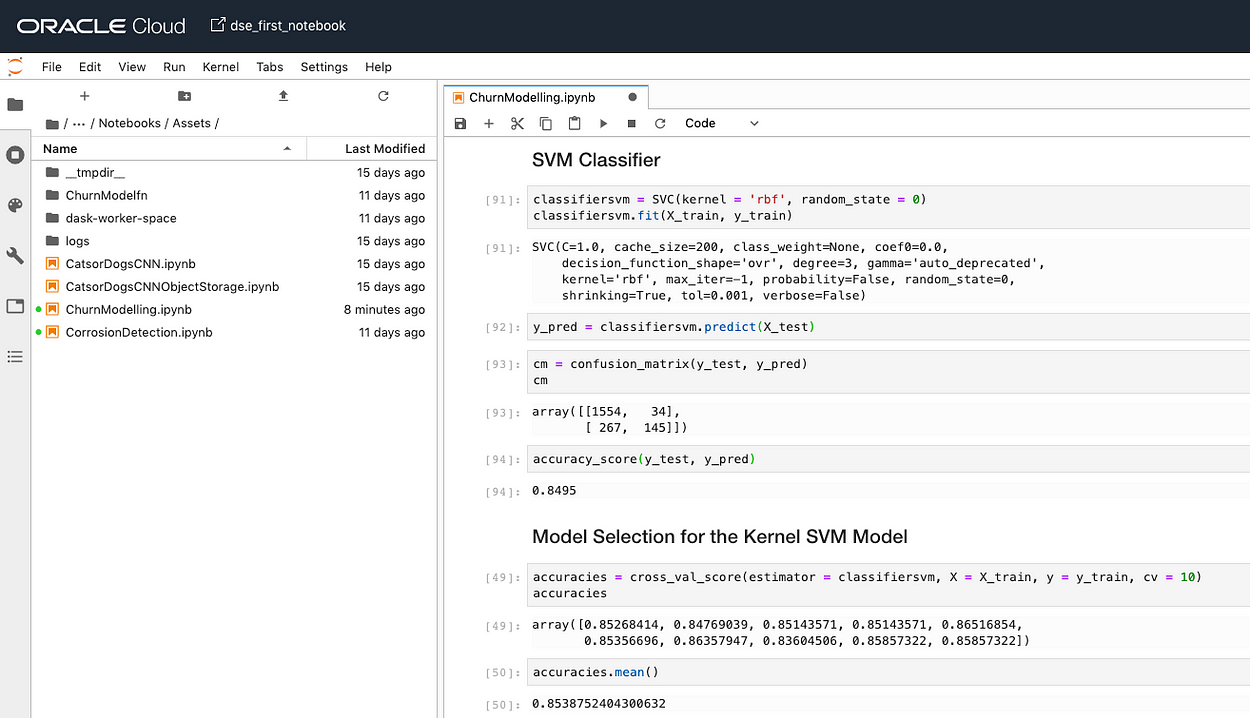
# Importing the librariesimport numpy as np
import matplotlib.pyplot as plt
import pandas as pdfrom sklearn.preprocessing import StandardScaler
from sklearn.svm import SVC
from sklearn.metrics import *
from sklearn.model_selection import cross_val_score
from sklearn.model_selection import train_test_split# Converting ADS Dataset object to Pandas Dataframe
dataset = ds.to_pandas_dataframe()
X = dataset.iloc[:,0:7].values
y = dataset.iloc[:,8].values# Splitting the dataset into the Training set and Test set
X_train, X_test, y_train, y_test = train_test_split(X, y, test_size = 0.2, random_state = 0)# Feature Scaling
sc = StandardScaler()
X_train = sc.fit_transform(X_train)
X_test = sc.transform(X_test)#SVM Classifier
classifiersvm = SVC(kernel = 'rbf', random_state = 0)
classifiersvm.fit(X_train, y_train)
y_pred = classifiersvm.predict(X_test)#Confusion Matrix
cm = confusion_matrix(y_test, y_pred)
cm
accuracy_score(y_test, y_pred)#K-fold Cross Validation
accuracies = cross_val_score(estimator = classifiersvm, X = X_train, y = y_train, cv = 10)
accuracies

6b. Using ADS Auto ML to build a prediction model

This is easy, we have already specified the target variable while data was loaded. AutoML can take many parameters such as time limit, min features, list of algorithms, mandatory features..etc.

from ads.automl.driver import AutoML
from ads.automl.provider import OracleAutoMLProvider
train, test = ds.train_test_split()
model, baseline = AutoML(train, provider= OracleAutoMLProvider()).train(model_list=["LGBMClassifier", "RandomForestClassifier"])

You can visualize the auto ml hyperparameter tuning trails using “automl.visualize_tuning_trials()”!

The output of the AutoML build gives us the best performing algorithm with features and the details of tuned hyperparameters.

So the 6 stage process of a custom model building is reduced down to a 2 stage process using AutoML.

7. Evaluate the Model

Evaluation can help machine learning developers to:

• Quickly compare models across several industry-standard metrics.

E.g., What’s the accuracy, and F1-Score of my binary classification model?

• Discover where a model is lacking in feedback into future model development.

E.g., While accuracy is high, precision is low, which is why the examples I care about are failing.

• Increase understanding of the trade-offs of various model types.

Evaluation can help end-users of machine learning algorithms to:

• Understand visually and numerically where the model is likely to perform well, and where it is likely to fail.

E.g., Model A performs well when the weather is clear but is much more uncertain during inclement conditions.

The ADS evaluations class comes in 3 flavors: Binary Classification, Multi-class Classification, and Regression.

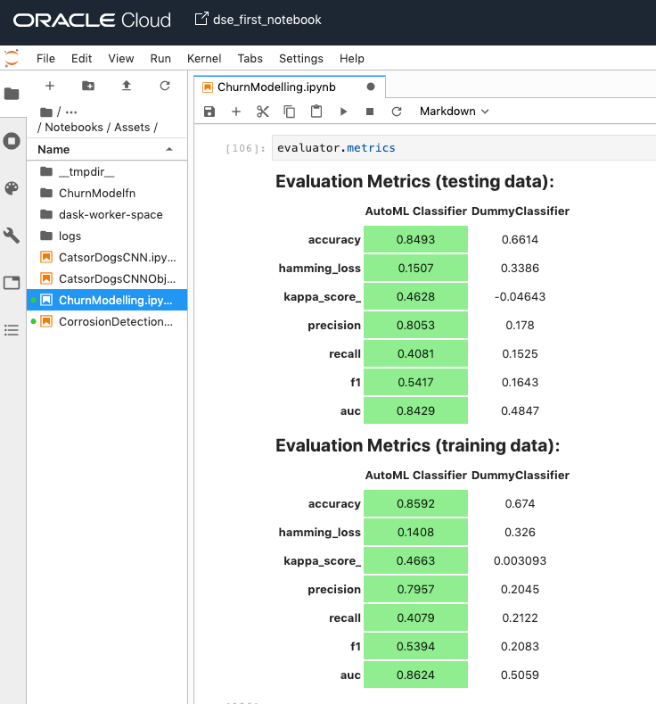
from ads.evaluations.evaluator import ADSEvaluator
from ads.common.data import MLData
evaluator = ADSEvaluator(test, models=[model, baseline], training_data=train)evaluator.metrics

“evaluator.show_in_notebook()” produces PR curve, ROC curve, Lift Chart, Gain Chart, and Confusion Matrix.

Why?

Machine learning explainability (MLX) is the process of explaining and interpreting machine learning and deep learning models.

Some useful terms for MLX:

• Explainability: The ability to explain the reasons behind a machine learning model’s prediction.
• Interpretability: The level at which a human can understand the explanation.
• Global Explanations: Understand the general behavior of a machine learning model as a whole.
• local Explanations: Understand why the machine learning model made a specific prediction.
• Model-Agnostic Explanations: Explanations treat the machine learning model (and feature pre-processing) as a black-box, instead of using properties from the model to guide the explanation.

The ADS explanation module provides interpretable, model-agnostic, local/global explanations.

But since the CIO was specific about a particular customer in the test set we need local explanations. “sample=31 is the customer z here”

Locally “age” has influenced the prediction outcome.

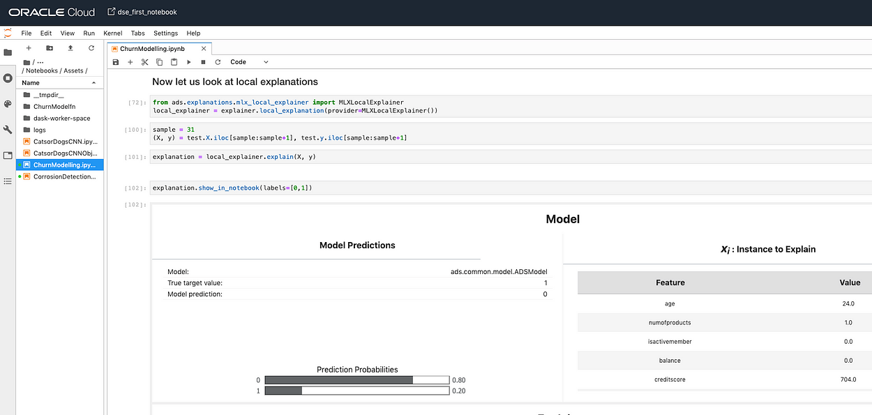
from ads.explanations.explainer import ADSExplainer
explainer = ADSExplainer(test, model, training_data=train)
from ads.explanations.mlx_global_explainer import MLXGlobalExplainer
global_explainer = explainer.global_explanation(provider=MLXGlobalExplainer())
importances = global_explainer.compute_feature_importance()
importances.show_in_notebook(n_features=7)from ads.explanations.mlx_local_explainer import MLXLocalExplainer
local_explainer = explainer.local_explanation(provider=MLXLocalExplainer())
sample = 31
(X, y) = test.X.iloc[sample:sample], test.y.iloc[sample:sample]
explanation = local_explainer.explain(X, y)
explanation.show_in_notebook(labels=[0,1])

I hope it was fun — If yes then my mission is accomplished!

Welcome to the world of Data Science done right!

Please don’t forget to clap if you liked this article 🙂

The views expressed are those of the author and not necessarily those of Oracle. Contact Deepak Sekar

Additional Resources

Overview — ADS 1.0.0 documentation

The Oracle Accelerated Data Science (ADS) SDK is a Python library that is included as part of the Oracle Cloud…

docs.cloud.oracle.com

Cloud Infrastructure for Data Science U+007C Oracle

No results found Your search did not match any results. We suggest you try the following to help find what you’re…

www.oracle.com

Data Science

Oracle Data Science is a platform for data scientists to build, train, and manage models on Oracle Cloud Infrastructure…

docs.cloud.oracle.com

Join thousands of data leaders on the AI newsletter. Join over 80,000 subscribers and keep up to date with the latest developments in AI. From research to projects and ideas. If you are building an AI startup, an AI-related product, or a service, we invite you to consider becoming a sponsor.

Published via Towards AI