Knowing Linear Regression better!!

Author(s): Charanraj Shetty

Originally published on Towards AI.

Statistics

OLS and Gradient Descent

Regression Introduction

Regression is an Algorithm of the Supervised Learning model. When the output or the dependent feature is continuous and labeled then, we apply the Regression Algorithm. Regression is used to find the relation or equation between the Independent variables and the output variable. E.g., given below, we have variable x₁, x₂, ….,xₙ, which contribute towards the output of variable y. We have to find a relation between x variables and dependent variable y. So the equation is defined as shown below, e.g.-

y = F( x₁, x₂, ….,xₙ)

y = 5 x₁+8x₂+….+12xₙ

To find a relation between independent features and dependent features in a better manner, we will reduce the independent feature to find an equation for the understanding purpose here.

Linear Regression

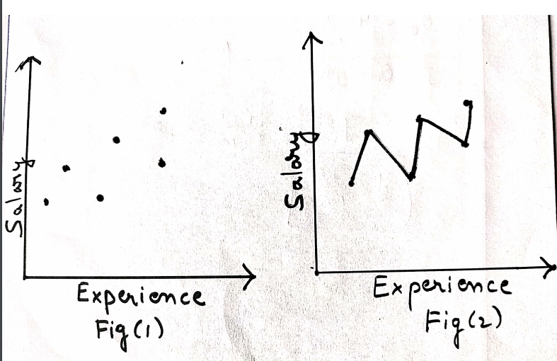
Assume that we want to calculate the salary based on the input variable Experience. So the salary becomes our independent feature x, and the experience becomes our dependent feature y.

Consider fig(1) in the above image where the value of y is increasing linearly with an increase in the value of x. It can be concluded that the dependency is linearly proportional. So the graph obtained is a straight line, and the relation between x and y is given y=2x+4.

Consider fig(2) in the above image where the value of y is not proportional to the increasing values of x. It's visible from fig(2) that the value of y is irregular w.r.t to y. So this type of regression is known as Non-Linear Regression.

With the above discussion, we must understand that life is not always going to be so smooth. Consider fig(1) in the below image where the points are spread across the plane. Is it possible to find the best fit line and the equation that passes through all the points in the plane? Yes, practically, it's possible, visible from fig(2) in the below image. But is it feasible? No, as it’s clearly visible from fig(2) that we are overfitting the data, this will compromise the model’s performance in terms of accuracy.

How do we avoid overfitting, and at the same time, we can find a line that passes through all the points? We select the best fit line that passes through all the points so that the distance of all the given points is minimum from the line, and we can find a relation between the output and input features by minimizing the error.

We plot all the points (x1,y1), (x2,y2),…..,(xₙ,yₙ) and calculate the error between the various lines which have been selected to obtain the best fit line. E.g. , in the below image, we have a point (x₁,y₁) which calculates the distance from the line (1) using the formula (Y₁-Ῡ)². Similarly, we calculate the distance of the second point (x₂,y₂) from the line(1) using the formula (Y2 – Ῡ)².In this way, we obtain the error difference of actual result and predicted result for each point from the (1) and then sum up the errors (1). Similarly, we calculate the sum of the value of errors for all the points from line(2), line(3), as our main goal is to minimize the error, so we focus on choosing the best fit line, which has points lying at minimum distance.

Once the line is obtained, we have the equation related to that line, which is denoted as Y = θ₀ + θ₁*X

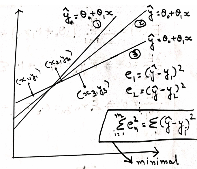
As we can observe from the above image, the main goal is to minimize the sum of errors between the actual and predicted value of the dependent variable. The equation is known as the Loss function. This process will, in turn, optimizes the value of θ₀ and θ₁, which will result in defining the best fit line that is having minimum distance from all the given points in space.

OLS Method

OLS (Ordinary Least Square) method is applied to find the linear regression model's values of parameters. We had derived the above equation Y = θ₀ + θ₁*X.

Revision of Maxima and Minima

Before we move ahead, let's understand the concept of engineering mathematics of Maxima and Minima. Points 1, 2, and 3 indicate where the slope changes its direction, either upward or downward. If you observe, it’s visible from the below figure that if we draw a tangent at points 1,2, and 3, it appears parallel to X-axis. So the slope at these points is 0. These points at which the slope becomes zero or are known as Stationary points. Also, point 1 in the below fig, where the slope's value suddenly starts increasing, is known as global minima, and vice-versa at point 2 is known as global maxima.

From the above concept, we can conclude that we can find the stationary points of any given equation by equating its derivative to zero, i.e., the slope at that point equal to zero. By solving the first derivative, we find the stationary points for the equation. But we need to conclude whether the stationary point is the global maxima or global minima.

On taking the second derivative, if the value is greater than zero, it represents global minima, and if the value is less than zero, it represents global maxima. In this way, we figure out the global maxima and minima.

We take the below example to understand the above rules about maxima and minima.

From all the above discussion, we can observe that it achieves minima when the graph attains a convex curve. Hence we can conclude that our point of discussion must be to attain convexity of the loss function.

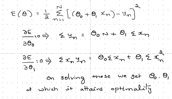
Optimization of θ₀ and θ₁

So we have a problem statement in the hand of optimizing the values θ₀ and θ₁ such that the Loss function attains convexity(minimum value). As we learned from the maxima and minima concept, we focus on obtaining the given loss function's stationary points, as shown below. Using that, we get two equations, as shown in the below image. Looking at both the equations, we know that ∑x ₙ, ∑ yₙ, ∑xₙyₙ, and ∑xₙ² can be obtained from the given data, which will have an independent variable salary(x) and dependent variable(y).

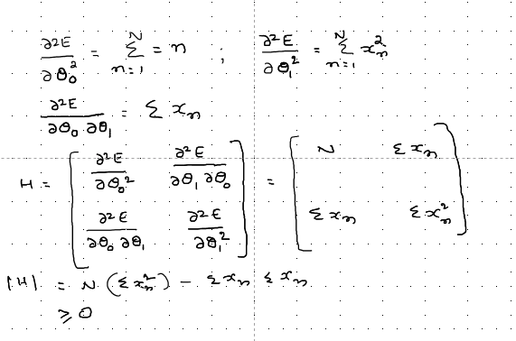
To take it a bit more forward, we can take the second derivative w.r.t θ₀ and θ₁ and form the Hessian matrix given in the below images.

Method to find out the convexity using the matrix

Although we found out the values of θ₀ and θ₁ at the stationarity point, we need to confirm now if the point of stationarity is convex or concave. To confirm the convexity of a matrix, we have a method given below:

Leading Principal Minor

If the matrix that corresponds to a principal minor is a determinant of the quadratic upper-left part of the larger matrix (i.e., it consists of matrix elements in rows and columns from 1 to k), then the principal minor is called a leading principal minor (of order k).

The kth order leading principal minor is the determinant of the kth order principal submatrix formed by deleting the last n − k rows and columns.

The principal leading minor of A is the submatrices formed from the first r rows and r columns of A for r=1,2,…..,n.

These submatrices are

Theorem:

A Symmetric matrix A is positive definite if and only if every leading principal minor's determinant is positive.

Example to understand the Principal Minor

Given below Matrix A and we form the Principal minors out of it. Once that is done, we take the value of the determinant.

If the value of Determinant of Principal Minors is greater than zero for all, then it's called positive definite (e.g., 2,3,1).

If the value of Determinant of Principal Minors is greater than or equal to zero for all, then it’s called positive semidefinite (e.g., 2,0,1).

If the value of Determinant of Principal Minors is less than zero for all, then it’s called negative definite (e.g., -2,-3,-1).

If the value of Determinant of Principal Minors is less than or equal to zero for all, then it’s called negative semidefinite (e.g., -2,0,-1).

As it is visible from the above image that the Principal minor determinant values are greater than zero, so it is positive.

Convexity of function

For a given matrix A,

A is convex ⇔ A is positive semidefinite.

A is concave ⇔ A is negative semidefinite.

A is strictly convex ⇔ A is positive definite.

A is strictly concave ⇔ A is negative definite.

Limitations of OLS

• If we observed the OLS method, then there are high chances of obtaining false-positive convex points, i.e., there might be two minimal in the same equation. One of them might be local minima while the other being global minima.
• Also, there isn't any fine-tuning parameter available to control the performance of the model. We aren't having control over the accuracy of the model. As we are targeting to build an optimized system, we must focus on controlling the model efficiency.

Gradient Descent Method

To overcome the OLS method's limitations, we introduce a new model for optimizing the values of θ₀ and θ₁, known as the Gradient Descent Method. Here we initialize the values of θ₀ and θ₁ to some random values and calculate the model output's total error. If the error is not within the permissible limits, we go for decrement of the θ₀ and θ₁ using the learning parameter α.

If we get the value of error in the model output higher in the present iteration compared to the previous iteration, then we might have possibly achieved convergence in the previous iteration. Or else we have another option of updating the value α and validate the output error. Here we take the derivative of Error function J(θ₀,θ₁) w.r.t θ₀ and θ₁ and use those values to obtain the new values of θ₀ and θ₁ in the next iteration.

This was all about the mathematical intuition behind Linear Regression, which helps us to know the concept better. One can get the methods to be used while performing the linear Regression from the Python packages easily.

Thanks for reading out the article!!

I hope this helps you with a better understanding of the topic.

Join thousands of data leaders on the AI newsletter. Join over 80,000 subscribers and keep up to date with the latest developments in AI. From research to projects and ideas. If you are building an AI startup, an AI-related product, or a service, we invite you to consider becoming a sponsor.

Published via Towards AI