


Improving Artificial Neural Network with Regularization and Optimization
Last Updated on December 15, 2020 by Editorial Team
Author(s): S.R. Shinde
In this article, we will discuss regularization and optimization techniques that are used by programmers to build a more robust and generalized neural network. We will study the most effective regularization techniques like L1, L2, Early Stopping, and Drop out which help for model generalization. We will take a deeper look at different optimization techniques like Batch Gradient Descent, Stochastic Gradient Descent, AdaGrad, and AdaDelta for better convergence of the neural networks.
Regularization for Model Generalization
Overfitting and underfitting are the most common problems that programmers face while working with deep learning models. A model that is well generalized to data is considered to be an optimal fit for the data. The problem of overfitting occurs when the model captures the noise of data. Precisely, overfitting occurs when a learning model has low bias and high variance. While in the case of underfitting the learning model can’t capture the inherent nature of data. The problem of underfitting persists when the model does not fit well on to the data. The underfitting problem reflects low variance and high bias.
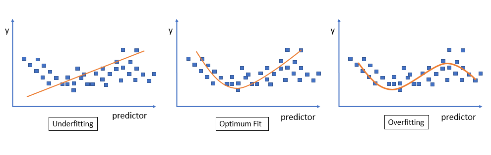
Regularization, in the context of neural networks, is a process of preventing a learning model from getting overfitted over training data. It involves a mechanism to reduce generalization errors of the learning model. Look at the following image which shows underfitting, which depicts the inability of a learning model to capture the inherent nature of data. This results in erroneous outcomes for unseen data. Also, we see overfitting over training data in the following image. This image also shows an optimum fit that presents the ability of a learning model to predict correct output for previously not seen data.
Generalization error is a scale to measure the ability of the learning model to correctly predict the response for unseen data. It can be minimized by avoiding overfitting over training data. L1, L2, Early stopping, and Drop Out are important regularization techniques to help improve the generalizability of a learning model.
Let’s discuss these techniques in detail.
L1 Regularization
Regularization is the process of preventing a learning model from getting overfitted over data. In L1 regularization, a penalty is introduced to suppress the learning model from getting overfitted. It introduces a new cost function by adding a regularization term in the loss function of the gradient of weights of the neural networks. With the addition of the regularization term, we penalize the loss function to an extent that it will get generalized.
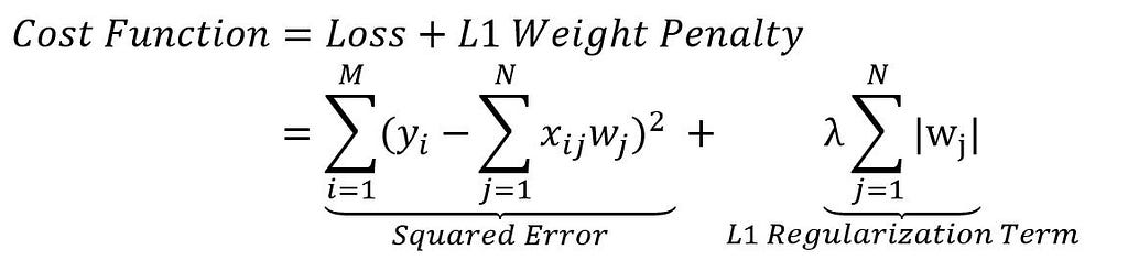
In this above equation, the L1 regularization term represents a magnitude of the coefficient value of the summation of the absolute value of weights or parameters of the neural network.
L2 Regularization
Similar to L1 regularization, L2 regularization introduces a new cost function by adding a penalty term to a loss function called an L2 weight penalty.
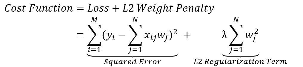
As shown in the above equation, the L2 regularization term represents the weight penalty calculated by taking the squared magnitude of the coefficient, for a summation of squared weights of the neural network. The larger the value of this coefficient, the higher is the penalty for complex features of a learning model.
Drop Out
A high number of nodes in each layer of a neural network capture the complex features of data along with noise which leads to overfitting of a learning model. In this regularization technique, the nodes are randomly selected and dropped to make a learning model more generalized so that it will perform better on newly arrived data as shown in the following diagram.
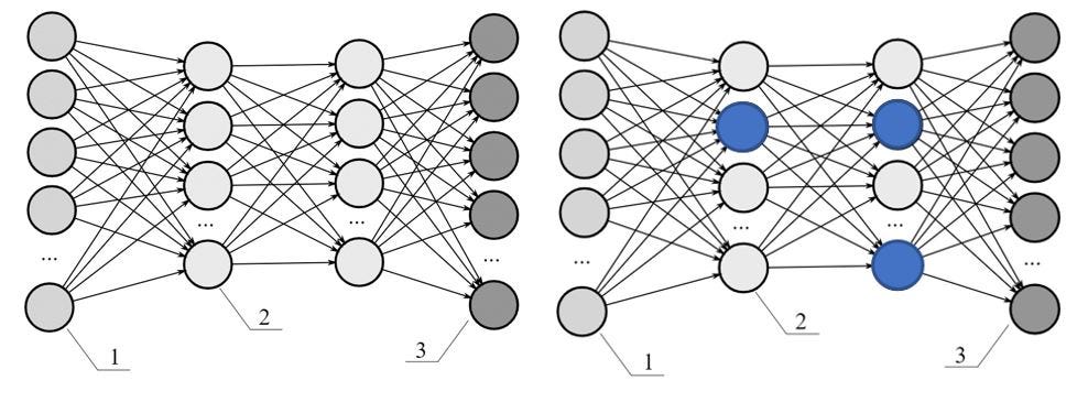
In the diagram above, the network on the left shows the fully connected dense neural network while the one on the right shows that few of the randomly selected nodes are dropped, which largely helps in preventing a learning model from getting overfitted on a training dataset and minimizes the regularization error.
Early Stopping
Early stopping is a type of regularization that’s used to avoid the overfitting of a learning model. A high number of training iterations or epochs leads to overfitting of the learning model over a dataset whereas a smaller number of epochs results in underfitting of the learning model. In early stopping, a neural network is simultaneously trained on training data and validated on testing data just to figure out how many iterations are needed for better convergence of the learning model before its validation error starts increasing as shown in the following figure.

In the case of neural networks, a learning model gets improved as we increase the number of training iterations to the point it may overfit the training data, in case if we don’t stop at an early stage. In this form of regularization, a model is being trained iteratively on the dataset with gradient descent until the validation error gets converged to minima. A learner’s performance can be further improved with a greater number of training iterations but at the expense of higher validation error. Early stopping determines how many iterations should a learner take for better accuracy taking into consideration that it should not overfit the training dataset. With early stopping, a neural network gets optimal weights for better convergence of learning with minimal generalization error.
Optimization for Model Performance
It is important to understand different optimization techniques like Batch Gradient Descent, Stochastic Gradient Descent, Mini-batch Gradient Descent, AdaGrad, AdaDelta for better convergence of the neural network.
Optimization techniques help in better convergence of a neural network by optimizing the gradient of the error function. There are many variants of gradient descent, which differentiate each other based on how much data is being processed to calculate the gradient of the error function (objective function). There exists a trade-off between the ability of the learning model in getting better converged on data and the computing resources needed to do that.
Batch Gradient Descent (Vanilla Gradient Descent)
Batch Gradient Descent is the most commonly used optimization algorithm for improving model performance. It uses the first-order approximation for finding minima for the objective function in an iterative manner. It uses a learning algorithm that updates the weights or parameters proportional to the negative of the gradient of the objective function for connections between layers of neurons in a multi-layered network.
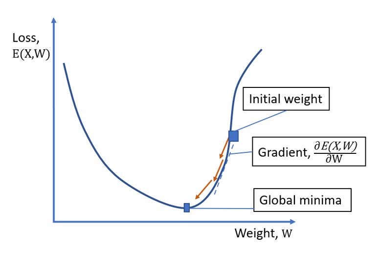
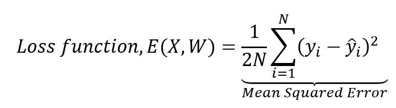
In other words, it tries to find out the optimal set of weights or parameters for the connections between different nodes of neural layers that will give a minimal error for the predictability. In the batch gradient descent, a loss function, as shown above in the diagram, is calculated by the aggregation of squared differences between correct response, y and calculated response, ŷ of all individual N data points, or observations in a dataset.
Once the loss function is calculated then weights for the neural networks are updated with the backpropagation algorithm, this is done iteratively until the loss function attains global minima.
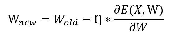
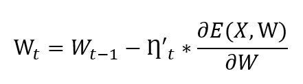
This above equation represents the weight updation formula in which represents old weights of the neural network while represents new weights for neural network updated with respect to the gradient of the loss function, with learning rate and set of data points, X. In short, a batch gradient descent considers all datapoints for loss computation in every iteration or epoch. The batch gradient descent outperforms with higher predictability of neural network but at the expense of computational time and resources.
Stochastic Gradient Descent
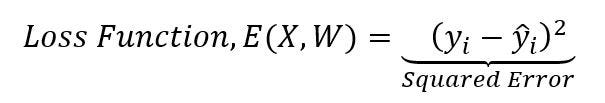
It’s a variant of gradient descent for model optimization. It considers only one datapoint or observation of a dataset in every iteration or epoch for calculation of loss function, E(X, W) as shown in the following equation,
It gives a similar performance like batch gradient descent but takes more time to converge due to frequent updates. Weights have high variance and make loss function to variate to different range of values.
Mini Batch Gradient Descent
Mini-batch gradient considers mini-batch of datapoints or observations of the dataset rather than considering all datapoints(as in batch gradient descent) or single datapoints(as in stochastic gradient descent), for calculation of loss function, over a mini-batch. It accordingly makes updations in the weights of connections between layers of neurons in the neural network.

In the above formula, K represents the size of the batch of data points of the dataset, N, taken into consideration for the calculation of loss function, over a K data points in every iteration or epoch. The mini-batch gradient descent variant helps to converge faster than stochastic gradient descent due to comparatively less frequent updates in the weights or parameters of neural network with lower variance in the loss function,
Adagrad
Adagrad (Adaptive Gradient) is a gradient-based optimization algorithm in which the learning rate updates with respect to the weights. It sets a low learning rate for the weights of connections between different layers of neurons in the neural network with commonly occurring features of data while setting it to a higher learning rate for the weights or parameters associated with uncommon features of data. Adagrad typically adapts different learning rates for every weight or parameter at every iteration or epoch based on their association with sparse or dense features. The weight updation formula in the adagrad is represented as follows,
In the above equation,ŋ_t represents an adaptive learning rate calculated with respect to the gradient of loss function at step t as follows,
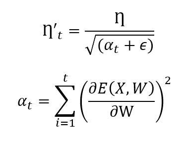
In the above equation, η represents a global learning rate and α_t represents the sum of squared gradients of past of loss functions, E(X, W) with ε, a small positive number. Whenever α_t increases to a higher bound, in turn, it reduces the learning rate drastically which affects the weight updation. To avoid this situation, Adadelta is the answer as discussed next in this section. The major benefit of using adaptive gradient optimization is that it removes the need for manual updation in the learning rate.
AdaDelta
Adadelta is an extended version of Adagrad that suppresses the aggressive growth of which in turn affects the learning rate. Adadelta updates the learning rate based on a sliding window of gradients of loss function rather than aggregating all past gradients.

Adadelta gives the adaptive learning rate based on gradient updates. Here in the above equation, W_avg represents the exponentially decaying average of squares of gradients which in turn helps to minimize the effects of past gradients which is calculated as follows,
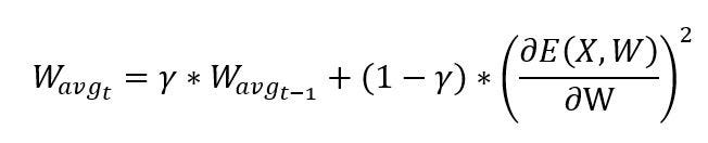
Initially, W is set to 0 for t = 0. The γ represents the Adadelta decay factor; it represents the fractional part of the gradient of the loss function to be kept in each time step, t. If it is set to a higher value, we could be able to restrict the growth of the gradient of loss function which in turn helps for better convergence of weights or parameters of neural network.
Summary
In this article, we learned different regularization techniques like L1, L2, drop out, and early stopping to prevent a learning model from getting overfitted on a training data and further to make a model more generalized for better predictability. We also learned different variants of gradient descent to obtain an optimal set of weights for connections between layers of nodes of a neural network. We studied different optimization techniques such as stochastic gradient descent, mini-batch gradient descent, adaptive gradient, adadelta for faster and smoother convergence of the gradient of the loss function, and to improve the accuracy of a learning model.
Improving Artificial Neural Network with Regularization and Optimization was originally published in Towards AI — Multidisciplinary Science Journal on Medium, where people are continuing the conversation by highlighting and responding to this story.
Published via Towards AI
Related posts


Comment (1)
Leave a Reply to Jaquavis Cancel reply
Popular posts

 for 2021")


Updates

Recent Posts


Jaquavis
Nice reading..