Image Gradient — Sobel Operator

Author(s): Vijay Vignesh

Originally published on Towards AI.

In my previous blog post, we explored the fundamental concept of Gaussian Blurring. Today, we will delve into another essential concept in classical computer vision known as Image Gradient. Image Gradient is the process of determining the rate of change of pixel intensities across an image. What exactly is the rate of change of pixel intensities and why is it helpful? The rate of change of pixel intensities refers to how much the pixel value changes in the vicinity of a specific pixel. It is useful in identifying the edges of objects in the image, which in turn is used extensively in many computer vision tasks like object detection and classification.

Let’s look at the picture below to gain a visual understanding of the concept. First, let’s look at the pixel highlighted in red. What is the rate of change of pixels? It is fairly low. If we look at its neighboring pixels (top, bottom, left, right), they are very close to their own value. On the contrary, the pixel highlighted in green tells a different story. It has a huge intensity drop going from bottom to top and also from right to left. This means that the rate of change of pixel values is high for that pixel. Can you notice the significance of the green pixel? Well, it marks the outer edge of the handwritten number ‘0’. This is exactly how we identify an edge. We analyze the gradient, or rate of change of pixel values, for each pixel, and those with higher gradients guide us to explore further.

Now that we understand the concept of an image gradient let’s explore the calculation process. The most popular way of calculating the image gradient is by using a Sobel filter. A filter, in this context, is basically a convolution operation applied to the image in order to extract specific features in the image. This convolution operation calculates a weighted sum of the pixel values, where the weights are defined by the values in the filter kernel. In my previous blog, I utilized a Gaussian filter. This time we’ll use a Sobel filter.

For each pixel, we slide the sobel_X and sobel_Y filters across each pixel of the image. Let’s look at sobel_X filter. The values on the left column are negative, middle column is zero and the right column is one. This means that sobel_X filter is searching for pixels where the values on the left side are significantly smaller than the values on the right side. Similarly, sobel_Y searches for areas where the top strip is drastically less than the bottom strip. Here’s a visualization of how sobel_X and sobel_Y filters work.

After obtaining the gradients in the perpendicular directions using the Sobel filter, we need to combine them to obtain the overall gradient. One of the key features of Sobel filters is that they allow us to calculate not only the magnitude of the gradient for each pixel but also its direction. To compute the magnitude, we square the x and y gradients at each pixel, sum them, and take the square root of the result. Finally, we can determine the direction of the gradient by dividing the y gradient by the corresponding x gradient at each pixel and taking the arctangent of the resulting value.

The code for the entire process is fairly straightforward. OpenCV has it all covered for us. It is important to note that Sobel filters are typically applied to grayscale images rather than RGB images. In the code snippet given below, line 2 applies the Sobel X filter, line 5 applies the Sobel Y filter, line 8 calculates the magnitude of the gradient at each pixel, and line 11 calculates the angle of the gradient. To ensure the output image is within the valid range, we normalize it in case any pixel value exceeds 255 or falls below 0.

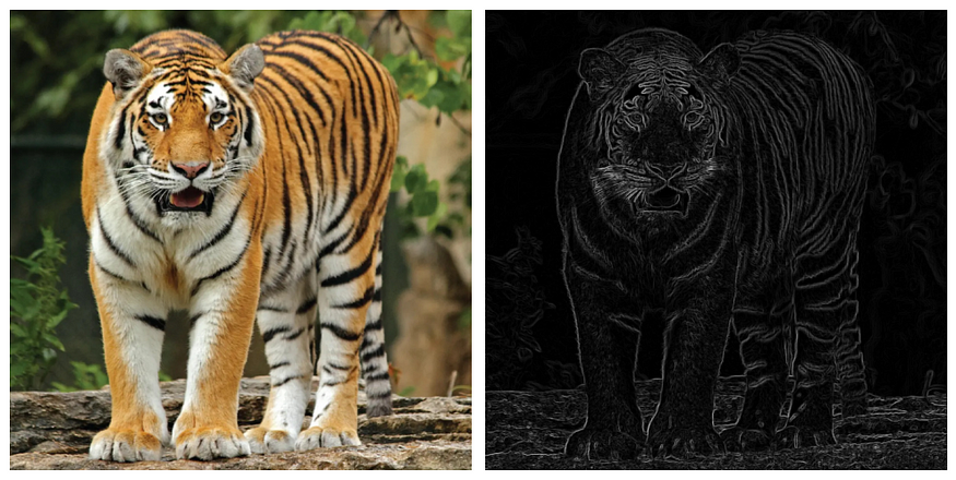
Finally, let’s visualize the output of the code above using a real-world image. I have used matplotlib to clearly display the outputs on a single plot.

That’s it, folks! Hopefully, now you have an idea about Image Gradients and how Sobel filters are used to obtain the Image Gradients. Stay tuned for more exciting topics in the realm of computer vision.

See you soon!

Join thousands of data leaders on the AI newsletter. Join over 80,000 subscribers and keep up to date with the latest developments in AI. From research to projects and ideas. If you are building an AI startup, an AI-related product, or a service, we invite you to consider becoming a sponsor.

Published via Towards AI