Gradient Descent v/s Normal Equation For Regression Problems

Author(s): Pushkara Sharma

Originally published on Towards AI.

Machine Learning

Choosing the right algorithm to find the parameters that minimize the cost function

In this article, we will see the actual difference between gradient descent and the normal equation in a practical approach. Most of the newbie Machine learning Enthusiasts learn about gradient descent during the linear regression and move further without even knowing about the most underestimated Normal Equation that is far less complex and provides very good results for small to medium size datasets.

If you are new to machine learning, or not familiar with a normal equation or gradient descent, don’t worry I’ll try my best to explain these in layman’s terms. So, I will start by explaining a little about the regression problem.

What is a Linear Regression?

It is the entry-level supervised (both feature and target variables are given) machine learning algorithms. Suppose, we plot all these variables in the space, then the main task here is to fit the line in such a way that it minimizes the cost function or loss(don’t worry I’ll also explain this). There are various types of linear regression like a simple(one feature), multiple, and logistic(for classification). We have taken multiple linear regression in consideration for this article. The actual regression formula is:-

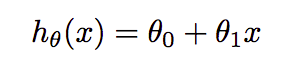
where θ₀ and θ₁ are the parameters that we have to find in such a way that they minimize the loss. In multiple regression, formula extended like θ₀+θ₁X₁+θ₂X₂. Cost function finds the error between the actual value and predicted value of our algorithm. It should be as minimum as possible. The formula for the same is:-

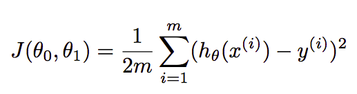
where m=number of examples or rows in the dataset, xᶦ=feature values of iᵗʰ example, yᶦ=actual outcome of iᵗʰ example.

Gradient Descent

It is an optimization technique to find the best combination of parameters that minimize the cost function. In this, we start with random values of parameters(in most cases zero) and then keep changing the parameters to reduce J(θ₀,θ₁) or cost function until end up at a minimum. The formula for the same is:-

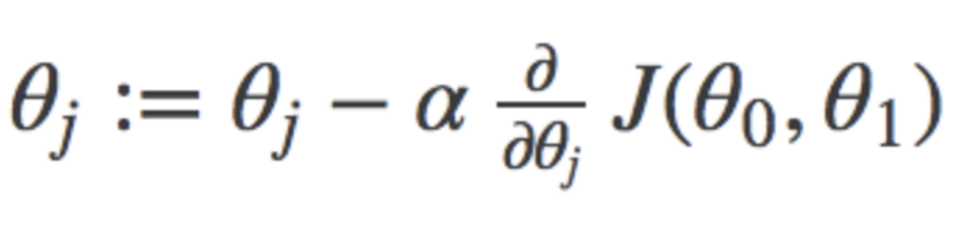
where j represents the no. of the parameter, α represents the learning rate. I will not discuss it in depth. You can find handwritten notes for these here.

Normal Equation

It is an approach in which we can directly find the best values of parameters without using gradient descent. It is a very effective algorithm or ill say formula(as it consists of only one line U+1F606)when you are working with smaller datasets.

The only problem with the normal equation is that finding the inverse of the matrix is computational very expensive in large datasets.

That’s a lot of theory, I know but that was required to understand the following code snippets. And I have only scratched the surface, so please google the above topics for in-depth knowledge.

Prerequisites:

I assume that you are familiar with python and already have installed the python 3 in your systems. I have used a jupyter notebook for this tutorial. You can use the IDE of your like. All required libraries come inbuilt in anaconda suite.

Let’s Code

The dataset that I have used consists of 3 columns, two of them are considered as features and the other one as the target variable. Dataset available in GithHub.

Firstly, we need to import the libraries that we will use in this study. Here, numpy is used to create NumPy arrays for training and testing data. pandas for making the data frame of the dataset and retrieving values easily. matplotlib.pyplot to plot the data like overall stock prices and predicted prices. mpl_toolkits for plotting 3d data, sklearn for splitting dataset and calculating accuracy. We have also imported time to calculate the time taken by each algorithm.

import pandas as pd
import numpy as np
from mpl_toolkits import mplot3d
import matplotlib.pyplot as plt
from sklearn.metrics import mean_squared_error
from sklearn.model_selection import train_test_split
import time

We have loaded the dataset into the pandas dataframeand the shape of dataset comes out to be (1000,3), then we simply print the first 5 rows with head() .

df = pd.read_csv('student.csv')
print(df.shape)
df.head()

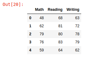
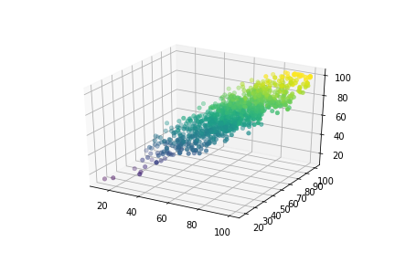
Here, feature values namely Math and Reading are saved in variables X1 and X2 as NumPy arrays whereas the Writing column is considered as a target variable and its values saved in the Y variable. Then we have plotted this 3D data.

X1 = df['Math'].values
X2 = df['Reading'].values
Y = df['Writing'].valuesax = plt.axes(projection='3d')
ax.scatter(X1, X2, Y, c=Y, cmap='viridis', linewidth=0.5);

Now, X₀ is initialized as a numpy array that consists of ones with the same dimensions as other features(It acts like bias). After that, we grouped all features in a single variable and transpose them to be in the right format. Then the data is split into training and testing with the help of train_test_split and test size was 5% that is 50 rows for testing. The shapes are given in the screenshot below.

X0 = np.ones(len(X1))
X = np.array([X0,X1,X2]).T
x_train,x_test,y_train,y_test = train_test_split(X,Y,test_size=0.05)
print("X_train shape:",x_train.shape,"\nY_train shape:",y_train.shape)
print("X_test shape:",x_test.shape,"\nY_test shape:",y_test.shape)

Here, Q denotes the list of parameters, which in our case are 3 (X₀, X₁, X₂), they are initialized as (0,0,0). n is just an integer with value equals to the number of training examples. Then we have defined our cost function that will be used in the gradient descent function to calculate the cost for every combination of parameters.

Q = np.zeros(3)
n = len(X1)
def cost_function(X,Y,Q):
 return np.sum(((X.dot(Q)-Y)**2)/(2*n))

This is the gradient descent function which takes features, target variable, parameters, epochs(number of iterations), and alpha(learning rate) as arguments. In the function, cost_history is initialized to append the cost of every combination of parameters. After that, we started a loop to repeat the process of finding the parameters. Then we calculated the loss and the gradient term and updated the set of parameters. Here, you don't see the partial derivative term because the formula here is used after computing partial derivate(for reference, see the square term in the formula described above is canceled out with 2 in the denominator). At last, we call cost function to calculate the cost and append it in the cost_history .

def gradient_descent(X,Y,Q,epochs,alpha):
 cost_history = np.zeros(epochs)
 for i in range(epochs):
 pred = X.dot(Q)
 loss = pred-Y
 gradient = X.T.dot(loss)/n
 Q = Q-gradient*alpha
 cost_history[i] = cost_function(X,Y,Q)
 return cost_history,Q

Here, we have started the timer before calling the above function and set epochs =1000 and alpha =0.0001(should be low as possible) and the timer stops just after the execution of the function. So our gradient descent takes around 82 milliseconds for execution(1000 epochs).

start = time.time()
cost_his,parameters = gradient_descent(x_train,y_train.flatten(),Q,1000,0.0001)
end = time.time()
print(end - start)

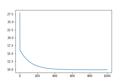
Here, we plotted the graph for cost_history . As we can see the graph converges at around 400 epochs, so I run the gradient descent function with epochs=400, and this time it takes around 25.3 milliseconds. You can test this yourself by using the notebook from my GitHub.

x = [i for i in range(1,1001)]
plt.plot(x,cost_his)

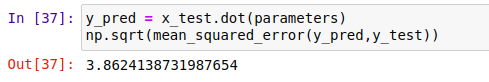
It is time for testing. The mean squared error comes out to be around 3.86 which is very acceptable.

y_pred = x_test.dot(parameters)
np.sqrt(mean_squared_error(y_pred,y_test))

Normal Equation

Normal Equation is very simple and you can see this in the code itself(only single line). As above, we have measured the time taken by the formula to calculate parameters. Don’t worry about the non-invertible matrix, NumPy covers all of them here. It takes around 3 milliseconds(average). Isn’t it great!

start = time.time()
Q1 = np.linalg.inv(x_train.T.dot(x_train)).dot(x_train.T).dot(y_train)
end = time.time()
print(end - start)

Finally, we have calculated the mean squared errorof Normal Equation which comes out to be 3.68

pred_y = x_test.dot(Q1)
np.sqrt(mean_squared_error(pred_y,y_test))

Conclusion

It turns out that Normal Equation takes less time to compute the parameters and gives almost similar results in terms of accuracy, also it is quite easy to use. According to me, the Normal Equation is better than Gradient Descent if the dataset size is not too large(~20,000). Due to the good computing capacity of today’s modern systems, the Normal Equation is the first algorithm to consider in cases of regression.

The source code is available on GitHub. Please feel free to make improvements.

Thank you for your precious time.U+1F60AAnd I hope you like this tutorial.

Also, check my tutorial on a Simple text summarizer.

Simple Text Summarizer Using Extractive Method

Automatically makes a small summary of the article containing the most important sentences.

towardsdatascience.com

Predict the Stock Trend Using Deep Learning

Predicting the upcoming trend of stock using Deep learning Model(Recurrent Neural Network)

medium.com

Join thousands of data leaders on the AI newsletter. Join over 80,000 subscribers and keep up to date with the latest developments in AI. From research to projects and ideas. If you are building an AI startup, an AI-related product, or a service, we invite you to consider becoming a sponsor.

Published via Towards AI