Gradient Descent Algorithm Explained

Last Updated on June 21, 2020 by Editorial Team

Author(s): Pratik Shukla

Machine Learning

With Step-By-Step Mathematical Derivation

Index:

• Basics Of Gradient Descent.
• Basic Rules Of Derivation.
• Gradient Descent With One Variable.
• Gradient Descent With Two Variables.
• Gradient Descent For Mean Squared Error Function.

What is Gradient Descent?

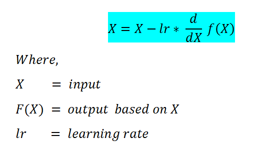
Gradient Descent is a machine learning algorithm that operates iteratively to find the optimal values for its parameters. It takes into account, user-defined learning rate, and initial parameter values.

How does it work?

• Start with initial values.
• Calculate cost.
• Update values using the update function.
• Returns minimized cost for our cost function

Why do we need it?

Generally, what we do is, we find the formula that gives us the optimal values for our parameter. But in this algorithm, it finds the value by itself! Interesting, isn’t it?

Formula:

Some Basic Rules For Derivation:

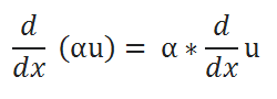
( A ) Scalar Multiple Rule:

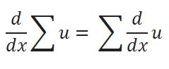
( B ) Sum Rule:

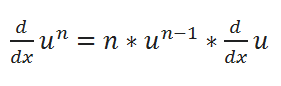
( C ) Power Rule:

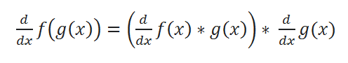
( D ) Chain Rule:

Let’s have a look at various examples to understand it better.

Gradient Descent Minimization — Single Variable:

We’re going to be using gradient descent to find θ that minimizes the cost. But let’s forget the Mean Squared Error (MSE) cost function for a moment and take a look at gradient descent function in general.

Now what we generally do is, find the best value of our parameters using some sort of simplification and make a function that will give us minimized cost. But here what we’ll do is take some default or random for our parameters and let our program run iteratively to find the minimized cost.

Let’s Explore It In-Depth:

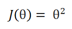
Let’s take a very simple function to begin with: J(θ) = θ², and our goal is to find the value of θ which minimizes J(θ).

From our cost function, we can clearly say that it will be minimum for θ= 0, but it won’t be so easy to derive such conclusions while working with some complex functions.

( A ) Cost function: We’ll try to minimize the value of this function.

( B ) Goal: To minimize the cost function.

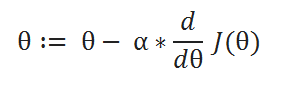
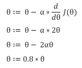
( C ) Update Function: Initially we take a random number for our parameters, which are not optimal. To make it optimal we have to update it at each iteration. This function takes care of it.

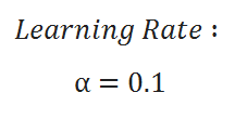
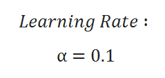
( D ) Learning rate: The descent speed.

( E ) Updating Parameters:

( F ) Table Generation:

Here we are stating with θ = 5.

keep in mind that here θ = 0.8*θ, for our learning rate and cost function.

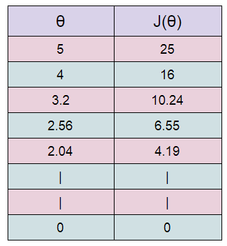
Here we can see that as our θ is decreasing the cost value is also decreasing. We just have to find the optimal value for it. To find the optimal value we have to do perform many iterations. The more the iterations, the more optimal value we get!

( G ) Graph: We can plot the graph of the above points.

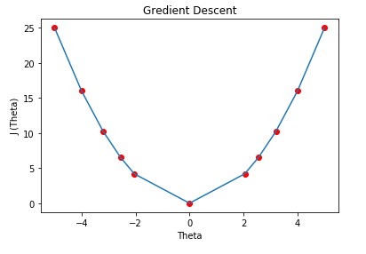
Cost Function Derivative:

Why does the gradient descent use the derivative of the cost function? We want our cost function to be minimum, right? Minimizing the cost function simply gives us a lower error rate in predicting values. Ideally, we take the derivative of a function to 0 and find the parameters. Here we do the same thing but we start from a random number and try to minimize it iteratively.

The learning rate / ALPHA:

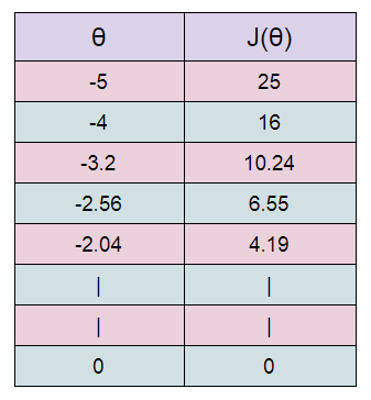
The learning rate gives us solid control over how large of steps we make. Selecting the right learning rate is a very critical task. If the learning rate is too high then you might overstep the minimum and diverge. For example, in the above example if we take alpha =2 then each iteration will take us away from the minimum. So we use small alpha values. But the only concern with using a small learning rate is we have to perform more iteration to reach the minimum cost value, this increases training time.

Convergence / Stopping gradient descent:

Note that in the above example the gradient descent will never actually converge to a minimum of theta= 0. Methods for deciding when to stop our iterations are beyond my level of expertise. But I can tell you that while doing assignments we can take a fixed number of iterations like 100 or 1000.

Gradient Descent — Multiple Variables:

Our ultimate goal is to find the parameters for MSE function, which includes multiple variables. So here we will discuss a cost function which as 2 variables. Understanding this will help us very much in our MSE Cost function.

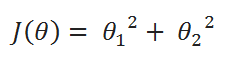
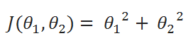
Let’s take this function:

When there are multiple variables in the minimization objective, we have to define separate rules for update function. With more than one parameter in our cost function, we have to use partial derivative. Here I simplified the partial derivative process. Let’s have a look at this.

( A ) Cost Function:

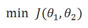
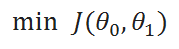
( B ) Goal:

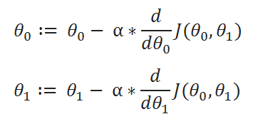
( C ) Update Rules:

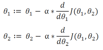
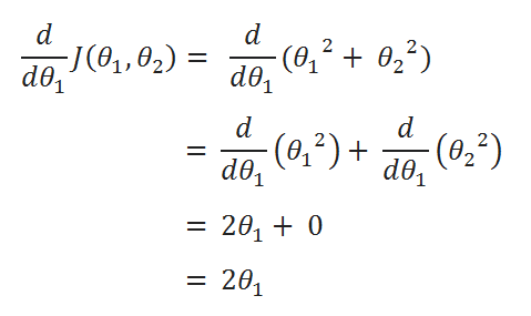
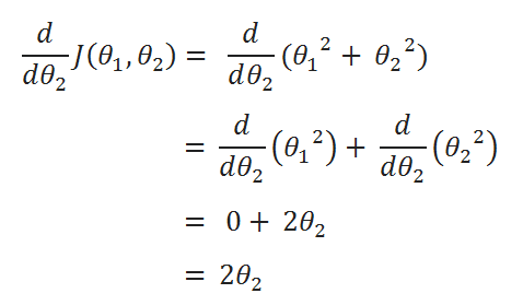
( D ) Derivatives:

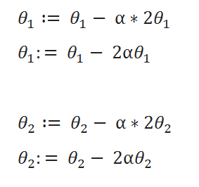
( E ) Update Values:

( F ) Learning Rate:

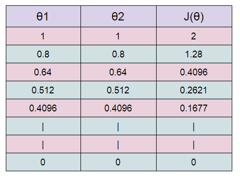
( G ) Table:

Starting with θ1 =1 ,θ2 =1. And then updating the value using update functions.

( H ) Graph:

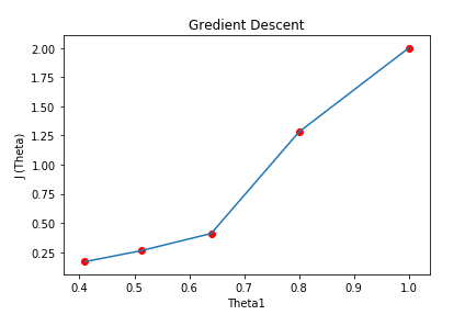
Here we can see that as we increase our number of iterations, our cost value is going down.

Note that while implementing the program in python the new values must not be updated until we find new values for both θ1 and θ2. We clearly don’t want to use the new value of θ1 to be used in the old value of θ2.

Gradient Descent For Mean Squared Error:

Now that we know how to perform gradient descent on an equation with multiple variables, we can return to looking at gradient descent on our MSE cost function.

Let’s get started!

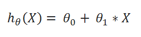
( A ) Hypothesis function:

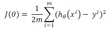
( B ) cost function:

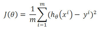
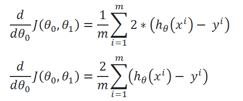
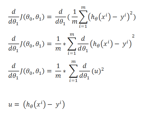
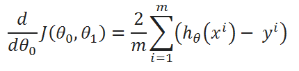
( C ) Find partial derivative of J(θ0,θ1) w.r.t to θ1:

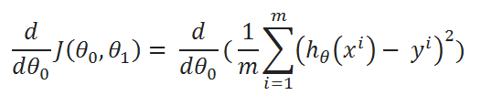
( D ) Simplify a little:

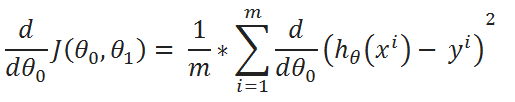
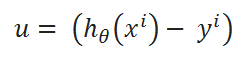
( E ) Define a variable u:

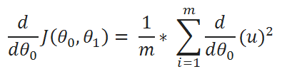
( F ) Value of u:

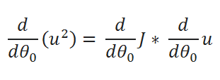
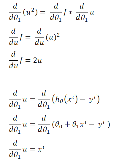
( G ) Finding partial derivative:

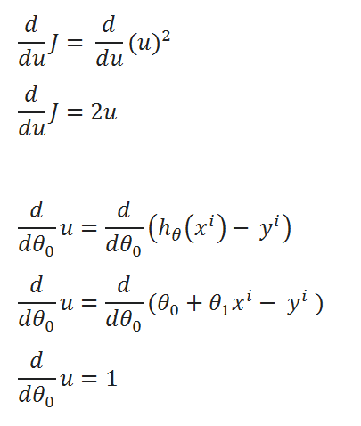
( H ) Rewriting the equations:

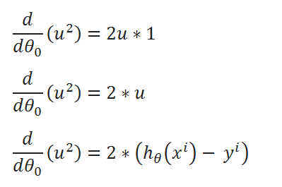
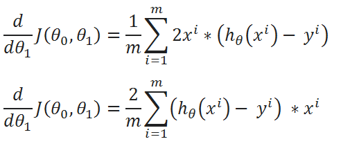
( I ) Merge all the calculated data:

( J ) Repeat the same process for derivation of J(θ0,θ1) w.r.t θ1:

( K ) Simplified calculations:

( L ) Combine all calculated Data:

One Half Mean Squared Error :

We multiply our MSE cost function with 1/2, so that when we take the derivative the 2s cancel out. Multiplying the cost function by a scalar does not affect the location of the minimum, so we can get away with this.

Final :

( A ) Cost Function: One Half Mean Squared Error:

( B ) Goal:

( C ) Update Rule:

( D ) Derivatives:

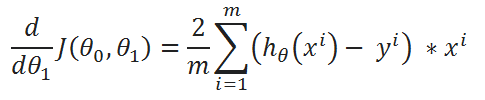
So, that’s it. We finally made it!

Conclusion:

We are going to use the same method in various applications of machine learning algorithms. But at that time we are not going to go in this depth, we’re just going to use the final formula. But it’s always good to know how it’s derived!

Final Formula:

Is the concept lucid to you now? Please let me know by writing responses. If you enjoyed this article then hit the clap icon.

If you have any additional confusions, feel free to contact me. [email protected]

---

Gradient Descent Algorithm Explained was originally published in Towards AI — Multidisciplinary Science Journal on Medium, where people are continuing the conversation by highlighting and responding to this story.

Published via Towards AI