


From Raw to Refined: A Journey Through Data Preprocessing — Part 2: Missing Values
Last Updated on August 9, 2023 by Editorial Team
Author(s): Shivamshinde
Originally published on Towards AI.
Before going through this article, please check out the previous article in the series on feature engineering.
From Raw to Refined: A Journey Through Data Preprocessing — Part 1: Feature Scaling
Sometimes, the data we receive for our machine learning tasks isn’t in a suitable format for coding with Scikit-Learn…
pub.towardsai.net
Why deal with missing values?
Most real word datasets come with at least some percent of missing values. But Scikit-Learn estimators do not work with such data. So to make the data compatible with the requirements of Scikit-Learn estimators, one has to deal with the missing values in the data.
Why completely removing the data records with missing values is a bad idea?
Dealing with missing values is a crucial part of data preprocessing. Often, the missing data is removed or imputed to handle this issue. However, completely removing missing values may not always be the best solution, especially when the dataset is small. This approach may lead to a further reduction in dataset size. Additionally, the missing data could be present due to specific conditions that were present during data collection, or it could be that the missing data exist in a particular pattern. Therefore, it is important to consider alternative methods for handling missing data.
Let me explain with an example. Imagine we are surveying college students, and one of the questions is about their weight. In this scenario, some female students may feel uncomfortable disclosing their weight due to societal expectations. As a result, we may encounter a high number of missing responses for weight among female participants. This is an example of missing data that follows a specific pattern.
Let’s examine another scenario from our survey. If we ask a question related to muscle strength or bicep size, many college-aged males might hesitate to provide their answers. This could be because they are self-conscious of their physical abilities or strength. As a result, we may end up with a significant number of missing responses from male participants.
Thus, almost always removing the records having missing values is a bad idea. This is because by doing this, we might forsake some useful information that is present in the data. A more sophisticated method for handling missing values involves filling in the gaps with a value obtained from other non-missing data.
Removing the columns with missing values could still give decent accuracy with large data. So, let’s see how to do this using code.
Handling missing value issue by removing the features that contain missing values
For the demonstration, we will use the Melbourne Housing Snapshot dataset from Kaggle. To keep things simple, we’ll only use the numerical features of the data.
## importing required libraries
import numpy as np
import pandas as pd
import matplotlib.pyplot as plt
import seaborn as sns

from sklearn.model_selection import train_test_split
from sklearn.ensemble import RandomForestRegressor
from sklearn.tree import DecisionTreeRegressor
from sklearn.metrics import mean_absolute_error

from sklearn.experimental import enable_iterative_imputer
from sklearn.impute import SimpleImputer, IterativeImputer, KNNImputer

import warnings
warnings.filterwarnings('ignore')
## reading the data
df = pd.read_csv('data-path')

## checking the basic information about the data
df.info()

## finding the names of numerical and categorical features
num_feat = [feature for feature in df.columns if df[feature].dtypes != 'O']
cat_feat = [feature for feature in df.columns if feature not in num_feat]

print(f"Numerical features: {num_feat}.\n")
print(f"Categorical features: {cat_feat}.")

## splitting the data into dependent feature ('Price') and independent features
X, y = df.drop('Price', axis=1), df['Price']

## removing the categorical features from data for simplicity.
X.drop(cat_feat, axis=1, inplace=True)
X.info()

## splitting the data into training data and validation data
X_train, X_valid, y_train, y_valid = train_test_split(X, y, train_size=0.8, test_size=0.2,
 random_state=0)
## checking the number of missing values in each of the features
missing_values_df = pd.DataFrame()
missing_values_df['Features'] = X_train.columns
missing_values_df['Number_of_missing_values'] = X.isnull().sum().to_numpy()
missing_values_df['Percentage_of_missing_values (%)'] = missing_values_df['Number_of_missing_values'].apply(lambda x: np.round((x/X_train.shape[0])*100),2)
missing_values_df

Let’s visualize the missing values in the data for fun.
import missingno as msgn

msgn.matrix(X_train)

In the above diagram, each white line represents a missing value, and black lines represent a non-missing value.
We can infer from the above diagram that the features, namely Car, BuildArea, and YearBuilt, contain missing values.
Now, let’s create a function that can be used to check how well the imputation methods are doing. We train a regressor on the imputed data and then find its mean absolute error value for an evaluation.
# Function for comparing different approaches
def score_dataset(X_train, X_valid, y_train, y_valid):
 model = RandomForestRegressor(n_estimators=10, random_state=0)
 model.fit(X_train, y_train)
 preds = model.predict(X_valid)
 return mean_absolute_error(y_valid, preds)
Now finally let’s remove the features having missing values.
# Get names of columns with missing values
cols_with_missing = [col for col in X_train.columns
 if X_train[col].isnull().any()]

# Drop columns in training and validation data
reduced_X_train = X_train.drop(cols_with_missing, axis=1)
reduced_X_valid = X_valid.drop(cols_with_missing, axis=1)

print(f"MAE from Approach of dropping columns with missing values:
 {np.round(score_dataset(reduced_X_train, reduced_X_valid, y_train, y_valid),2)}")

Another approach to handling the missing value problem is to fill the gaps with some value.
How to handle missing data through imputation

There are mainly two ways to impute the missing values using Scikit-Learn library classes namely Univariate feature imputation and Multivariate feature imputation.
In univariate feature imputation, the value needed for imputation is calculated using the data present in the single feature. For example, if one desires to impute the missing value in the weight column, then the value for imputation is calculated using the non-missing values of the weight column.
In multivariate feature imputation, the value needed for imputation is calculated using the data present in more than one feature. For example, to impute the missing values present in the weight column, the non-missing values from other columns, such as height and bicep size, can also be used.
Univariate Feature Imputation
Scikit-Learn SimpleImputer class is used to perform univariate feature imputation. The SimpleImputer class enables us to replace missing values with a constant value we choose or statistical values like the mean, median, or mode of the non—missing data in the same column.
SimpleImputer parameters
Scikit-Learn SimpleImputer has four important parameters, namely missing_values, strategy, fill_value, and add_indicator.
missing_values: This parameter indicates the placeholder for missing values in data, commonly set as numpy.nan.
strategy: This parameter is used to show the strategy that is used for imputation. There are four strategies available for SimpleImputer class namely mean, median, most_frequent aka mode, and a constant.
fill_value: When strategy = ‘most_frequent’, then we need to assign the constant value to the fill_value parameter.
add_indicator: This parameter is useful when the missing values show some kind of pattern. If add_indicator = True then, for every column containing missing values, a new column is created. For each new column, a value of 1 is placed at the index, where a missing value is found in the original column, and a value of 0 is placed everywhere else.
SimpleImputer Code Demonstration
Now, let’s see how to perform the imputation using SimpleImputer class.
si = SimpleImputer(missing_values=np.nan, strategy='mean', add_indicator=True)

print(f"Data before imputation of missing values in X_train:\n\n {X_train.head()}\n\n")
print(f"Column names of X_train before imputation:\n\n {X_train.columns.values}\n\n")

filled_X_train = pd.DataFrame(si.fit_transform(X_train), columns=si.get_feature_names_out())
filled_X_valid = pd.DataFrame(si.transform(X_valid), columns=si.get_feature_names_out())

print(f"Data after imputation of missing values in X_train:\n\n {filled_X_train.head()}\n\n")
print(f"Column names of X_train after imputation:\n\n {filled_X_train.columns.values}\n\n")

print(f"MAE for the imputation approach of using SimpleImputer: {np.round(score_dataset(filled_X_train, filled_X_valid, y_train, y_valid),2)}")
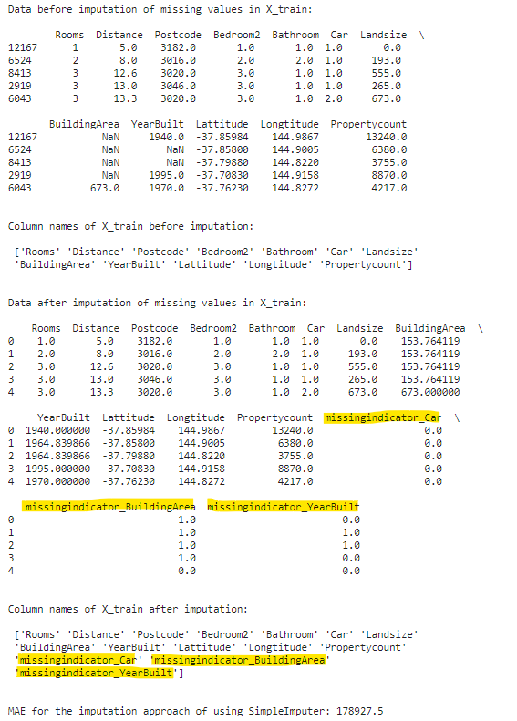
Please note that three additional columns (marked in yellow color) have been added to the data set following imputation because we set add_indicator = True. There were initially three columns with missing values, and to retain the missing value patterns within each of those three columns, three new columns were created.
Which strategy to use
Also, another important factor related to the SimpleImputer is knowing which strategy to use. The strategy is mainly based on the type of data and the presence of outliers in the data.
strategy = ‘mean’ is used when the data is numerical and free of any outliers.
strategy = ‘median’ is used when the data is numerical and with outliers.
strategy = ‘most_frequent’ is used for the categorical data.
strategy = ‘constant’ is used when the data is categorical or when we want to fill the missing values with a custom value.
Multivariate Feature Imputation
There are two choices for us in multivariate feature imputation in Scikit — learn namely IterativeImputer and KNNImputer.
Let’s understand the IterativeImputer first.
IterativeImputer
Please take note that this estimator is currently in an experimental state. As a result, the code with IterativeImputer may potentially break in the future.
In IterativeImputer, the feature with missing values is considered a dependent feature, and all the other columns as independent features. Then the regressor is trained on non-missing values of dependent features. The trained model will then predict the missing values in the dependent column. This is repeated for every column that contains missing values.
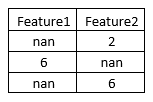
Let’s take an example to understand this more clearly. Let’s say our train and test data are as follows.

If we want to impute the missing values in Feature2 then, IterativeImputer will create a function as follow:

IterativeImputer thus will create a regressor with Feature2 as ‘y’ and Feature1 as ‘X’. Once the model is trained in such a way, it will discover that the values in Feature2 are twice that of values in Feature1. Using this logic, the missing values in Feature2 are imputed.
Likewise, another model will be trained to impute the values in Feature1.
Now, let’s see how to implement IterativeImputer.
iterimputer = IterativeImputer(estimator=DecisionTreeRegressor(), missing_values=np.nan, add_indicator=True)

print(f"Data before imputation of missing values in X_train:\n\n {X_train.head()}\n\n")
print(f"Column names of X_train before imputation:\n\n {X_train.columns.values}\n\n")

filled_X_train = pd.DataFrame(iterimputer.fit_transform(X_train), columns=iterimputer.get_feature_names_out())
filled_X_valid = pd.DataFrame(iterimputer.transform(X_valid), columns=iterimputer.get_feature_names_out())

print(f"Data after imputation of missing values in X_train:\n\n {filled_X_train.head()}\n\n")
print(f"Column names of X_train after imputation:\n\n {filled_X_train.columns.values}\n\n")

print(f"MAE for the imputation approach of using IterativeImputer: {np.round(score_dataset(filled_X_train, filled_X_valid, y_train, y_valid),2)}")
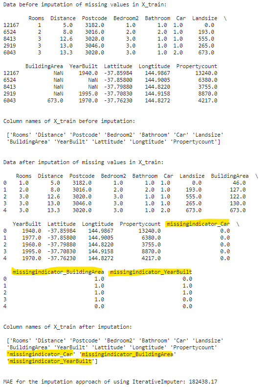
Please note that we can also specify which regressor to use for the imputation using the estimator parameter of IterativeImputer. Also, IterativeImputer has an add_indicator parameter and it works exactly like the one in SimpleImputer.
KNNImputer
This imputer uses the concept of K-nearest neighbors. The euclidean distance namely nan_euclidean_distances, which supports the missing values, is used to calculate the distance.
Let’s see how the nan_euclidean_distances work. When calculating the distance between pair of samples, this formulation ignores the feature coordinates with missing values in either sample and scales up the weight of the remaining coordinates.

While calculating the distance we take the coordinates where either values are not missing i.e., a1, a2,.. and b1, b2,… are not missing values.
Now, let’s take an example to understand how this algorithm works.
Consider the following data.

Let’s say we want to impute the missing value present at the first index in Feature1.
STEP 1:
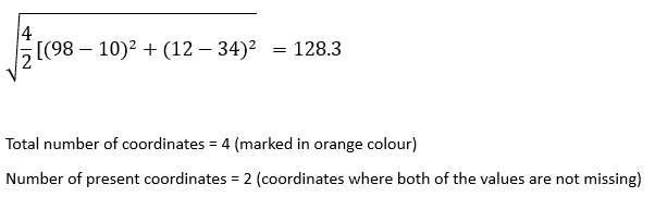
we will find out the distance nan_euclidean_distance between every row record and the row record at index 1.
nan_euclidean_distance between the record at index 1 and the record at index 2:

Similarly,
nan_euclidean_distance between the record at index 1 and the record at index 3:
nan_euclidean_distance between the record at index 1 and the record at index 4:

nan_euclidean_distance between the record at index 1 and the record at index 5:
STEP 2:
In this step, we will sort these distances in ascending order.
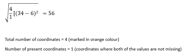
56, 128.3, 159.8, 193.8
STEP 3:
In this step, will take the first K (K value in K nearest neighbors) number of values in our order.
If K = 2, then we will impute the missing value with the average of the first two values in order, i.e., (56 + 128.3) / 2 = 92.15
If K = 3 then we will impute the missing value with the average of the first three values in order, i.e., (56 + 128.3 + 159.8) / 3 = 114.7
as so on.
Now that we have learned how the algorithm works, let’s see how to implement it.
knnimputer = KNNImputer(n_neighbors=3, missing_values=np.nan, add_indicator=True)

print(f"Data before imputation of missing values in X_train:\n\n {X_train.head()}\n\n")
print(f"Column names of X_train before imputation:\n\n {X_train.columns.values}\n\n")

knn_filled_X_train = pd.DataFrame(knnimputer.fit_transform(X_train), columns=knnimputer.get_feature_names_out())
knn_filled_X_valid = pd.DataFrame(knnimputer.transform(X_valid), columns=knnimputer.get_feature_names_out())

print(f"Data after imputation of missing values in X_train:\n\n {knn_filled_X_train.head()}\n\n")
print(f"Column names of X_train after imputation:\n\n {knn_filled_X_train.columns.values}\n\n")

print(f"MAE for the imputation approach of using KNNImputer: {np.round(score_dataset(knn_filled_X_train, knn_filled_X_valid, y_train, y_valid),2)}")

Note that IterativeImputer also has an add_indicator parameter, and it works exactly like the one in SimpleImputer.
Thanks for reading! If you have any thoughts on the article, then please let me know.
Are you struggling to choose what to read next? Don’t worry, I know of an article that I believe you will find interesting.
Be Confident in your Machine Learning Models with the help of Cross-Validation
Cross-validation is a go-to tool to check if your machine-learning model is reliable enough to work on new data. This…
pub.towardsai.net
and one more…
From Chaos to Order: Harnessing Data Clustering for Enhanced Decision-Making
This article will show the important use cases of data clustering methods, how to use these methods, and also show how…
pub.towardsai.net
Shivam Shinde
Have a great day!
Join thousands of data leaders on the AI newsletter. Join over 80,000 subscribers and keep up to date with the latest developments in AI. From research to projects and ideas. If you are building an AI startup, an AI-related product, or a service, we invite you to consider becoming a sponsor.
Published via Towards AI
Towards AI Academy
We Build Enterprise-Grade AI. We'll Teach You to Master It Too.
15 engineers. 100,000+ students. Towards AI Academy teaches what actually survives production.
Start free — no commitment:
→ 6-Day Agentic AI Engineering Email Guide — one practical lesson per day
→ Agents Architecture Cheatsheet — 3 years of architecture decisions in 6 pages
Our courses:
→ AI Engineering Certification — 90+ lessons from project selection to deployed product. The most comprehensive practical LLM course out there.
→ Agent Engineering Course — Hands on with production agent architectures, memory, routing, and eval frameworks — built from real enterprise engagements.
→ AI for Work — Understand, evaluate, and apply AI for complex work tasks.
Note: Article content contains the views of the contributing authors and not Towards AI.
Related posts
Recent Posts


")


