Exploratory Data Analysis (EDA) — Don’t ask how, ask what

The first step in any data science project is EDA. This article will explain why each step in the EDA is important and why we should care about what we learn from our data.

This is part 1 in a series of articles guiding the reader through an entire data science project (if you’re ready, you can skip to part 2 — Preparing your Dataset for Modelling — here)

I am a new writer on Medium and would truly appreciate constructive criticism in the comments below.

Overview

What is EDA anyway?

EDA or Exploratory Data Analysis is the process of understanding what data we have in our dataset before we start finding solutions to our problem. In other words — it is the act of analyzing the data without biased assumptions in order to effectively preprocess the dataset for modeling.

Why do we do EDA?

The main reasons we do EDA are to verify the data in the dataset, to check if the data makes sense in the context of the problem, and even sometimes just to learn about the problem we are exploring. Remember:

What are the steps in EDA, and how should I do each one?

• Descriptive Statistics — get a high-level understanding of your dataset
• Missing values — come to terms with how bad your dataset is
• Distributions and Outliers — and why countries that insist on using different units make our jobs so much harder
• Correlations — and why sometimes even the most obvious patterns still require some investigating

A note on Pandas Profiling

Pandas Profiling is probably the easiest way to do EDA quickly (although there are many other alternatives such as SweetViz ). The downside of using Pandas Profiling is that it can be slow to give you a very in-depth analysis, even when not needed.

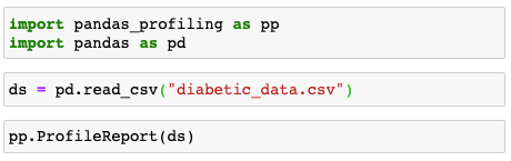
I will describe below how I used Pandas Profiling for analyzing the Diabetics Readmission Dataset on Kaggle (https://www.kaggle.com/friedrichschneider/diabetic-dataset-for-readmission/data)

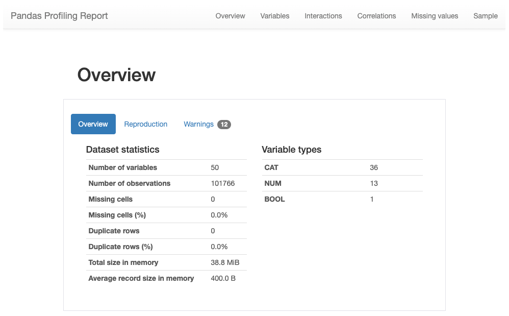
To see the Pandas Profiling report, simply run the following:

Descriptive Statistics

For this stage, I like to look at just a few key points:

• I look at the count to see if I have a significant amount of missing values for each specific feature. If there are many missing values for a certain feature I might want to discard it.

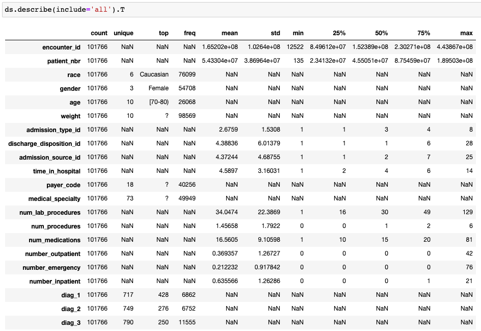
• I look at the unique values (for categorical, this will show up as NaN for pandas describe, but in Pandas Profiling, we can see the distinct count). If a feature has only 1 unique value it will not help my model, so I discard it.

• I look at the ranges of the values. If the max or min of a feature is significantly different from the mean and from the 75% / 25%, I might want to look into this further to understand if these values make sense in their context.

Missing Values

Almost every real-world dataset has missing values. There are many ways to deal with missing values — usually the techniques we use depend on the dataset and the context. Sometimes we can made educated guesses and/or impute the values. Instead of going through all the each method (there are many great medium articles out there describing the different methods in depth — see this great article by Jun Wu ), I will discuss how, sometimes, even though we are given a value in the data, the value is actually missing, and one particular method that allows us to ignore the hidden values for the time being.

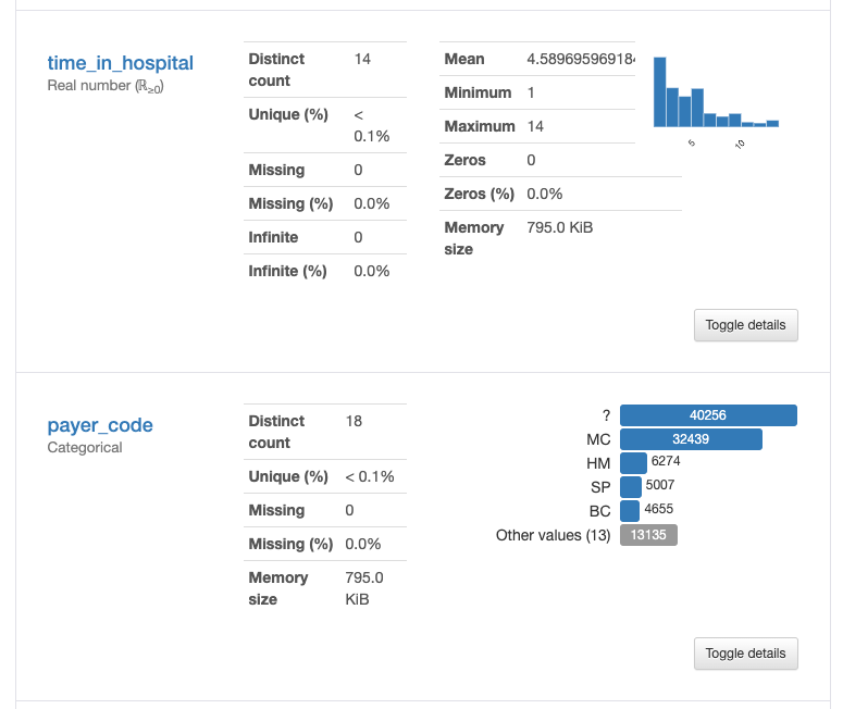
The diabetes dataset is a great example of missing values hidden within the data. If we look at the ‘descriptive statistics’ we can see zero missing values, but a simple observation of one of the features, in this case, “payer_code” in the figure above, we can see that almost half of the samples have a category “?”. These are hidden missing values.

What should we do when half the samples have missing values? There is no one right answer (See Jun Wu’s article). Many would say just exclude the feature with many missing values from your model as there is no way to accurately impute them.

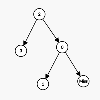
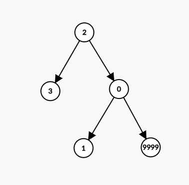
But there is one method many data scientists miss out on. If you are using a Decision Tree-based model (such as a GBM), then the tree can take a missing value as an input. Since all features will be turned into numeric values we can just encode “?” as an extreme value that is far from the range used in the dataset (such as 999,999), this way at the node, all samples with missing values will split to one side of the tree. If we find after modeling that this value is very important, we can come back to the EDA stage and try and understand (probably by using a domain expert) if there is valuable information in all the missing values of this specific feature. Some packages don’t even require you to encode missing values, such as LightGBM which automatically does this split.

Duplicate Rows

Duplicate rows sometimes appear in datasets. It is very easy to solve (this is one solution using the pandas build-in method):

df.drop_duplicates(inplace=True)

There is another type of duplicate rows that you need to be wary of. Say you have a dataset on patients. You might have many rows for each patient that represent taking a medication. These are not duplicates. We will explore how to deal with this kind of duplicate rows later in the series when we explore ‘Feature Engineering’.

Distributions and Outliers

The main reason to analyze the distributions and outliers in the dataset is to validate that the data is correct and makes sense. Another good reason to do this is to simplify the dataset.

Validating the Dataset

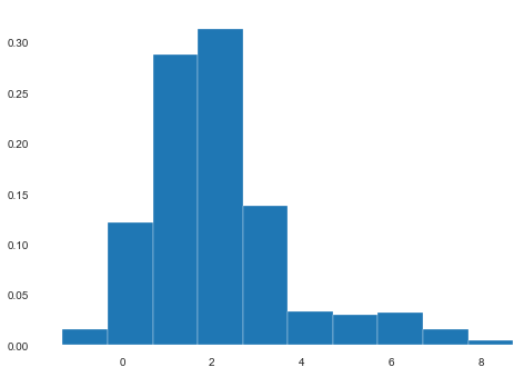
Let’s say we plot a histogram for the heights of the patient and we observe the following

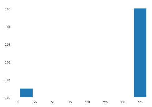
Clearly there is some kind of problem with the data. Here we can guess (due to the context) that 10% of the data has been measured in feet, and the rest in centimeters. We can then convert the rows where the height is less than 10 from feet to centimeters. Pretty simple. What do we do in a more complicated example, such as the one below?

Here, if we briefly look at the dataset and don’t check each and every feature, we will miss that patients’ heights are recorded as tall as even 6 meters, which doesn’t make sense (see Tallest People in the World). To solve this unit error, we must make some decisions on the cutoff: which heights are measured in feet and which in meters. Another option is to check if there is a correlation between height and country, for example, and we might find that all the feet measurements are from the US.

Outliers

Another important thing is to check outliers. We can graph the different features either as box-plots or as a function of another feature (typically the target variable, but not necessarily). There are many statistics to check for outliers in the data, but often in EDA, we can identify them very easily. In the example below, we can immediately identify outliers (random data).

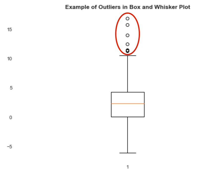
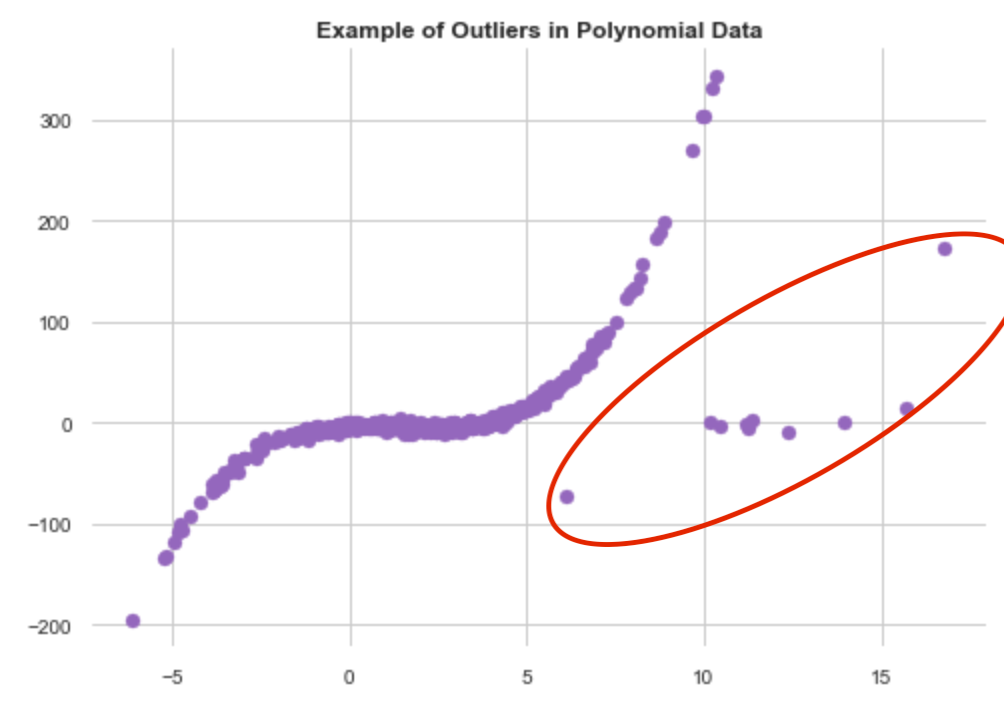
It is important to check outliers to understand if these are errors in the dataset. This is a whole separate topic (See Natasha Sharma’s excellent article on the topic), but a very important one to understand whether or not to keep there are errors in the dataset.

Simplifying the Dataset

Another really important reason to do EDA is that we might want to simplify our dataset and or even just identify where to simplify the dataset.

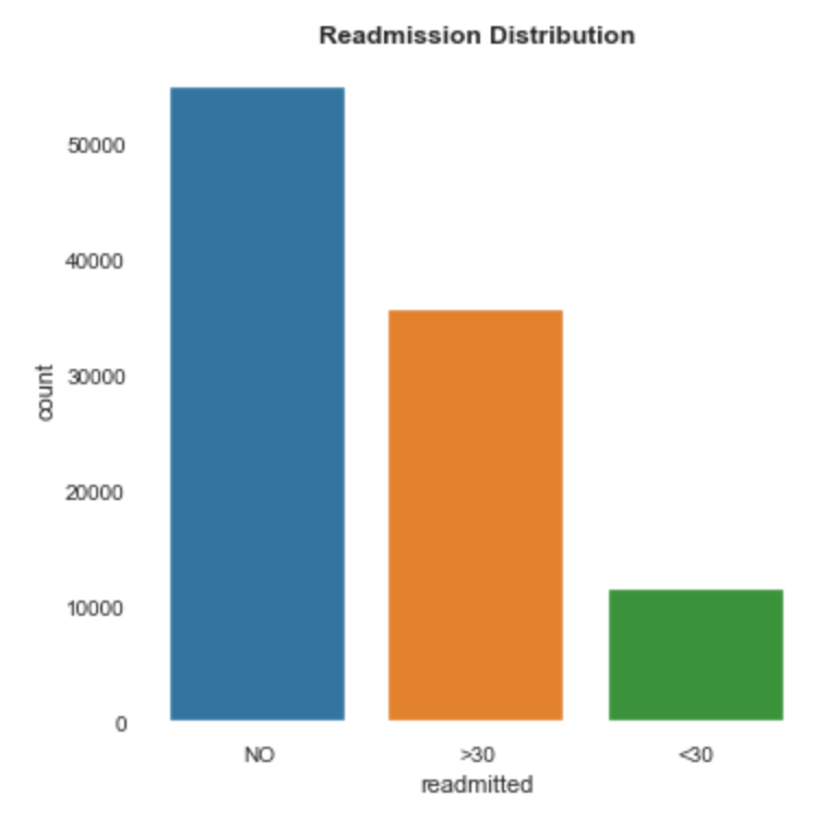
Perhaps we can group certain features in our dataset? Take the target variable “Readmission” in the diabetes patient dataset. If we plot the different variables we find that readmission in under 30 days and in over 30 days, generally follows the same distribution across different features. If we merge them we can balance our dataset and get better predictions.

If we check the distribution against different features we find that this still holds, take for example across genders

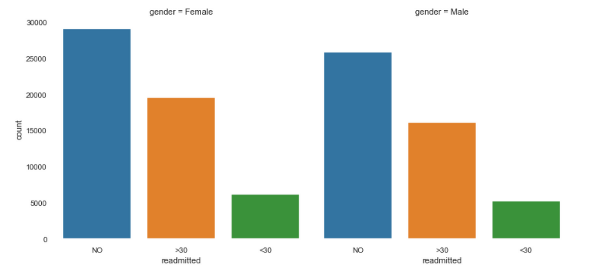
We can check this across different features, but here the conclusions seem to be that the dataset is very balanced and we can probably combine ‘readmitted’ in over or under 30 days.

Learn the Dataset

Another very important reason to visualize the distributions of your datasets is to learn what you even have. Take the following population pyramid of ‘Patient Numbers’ by age and gender

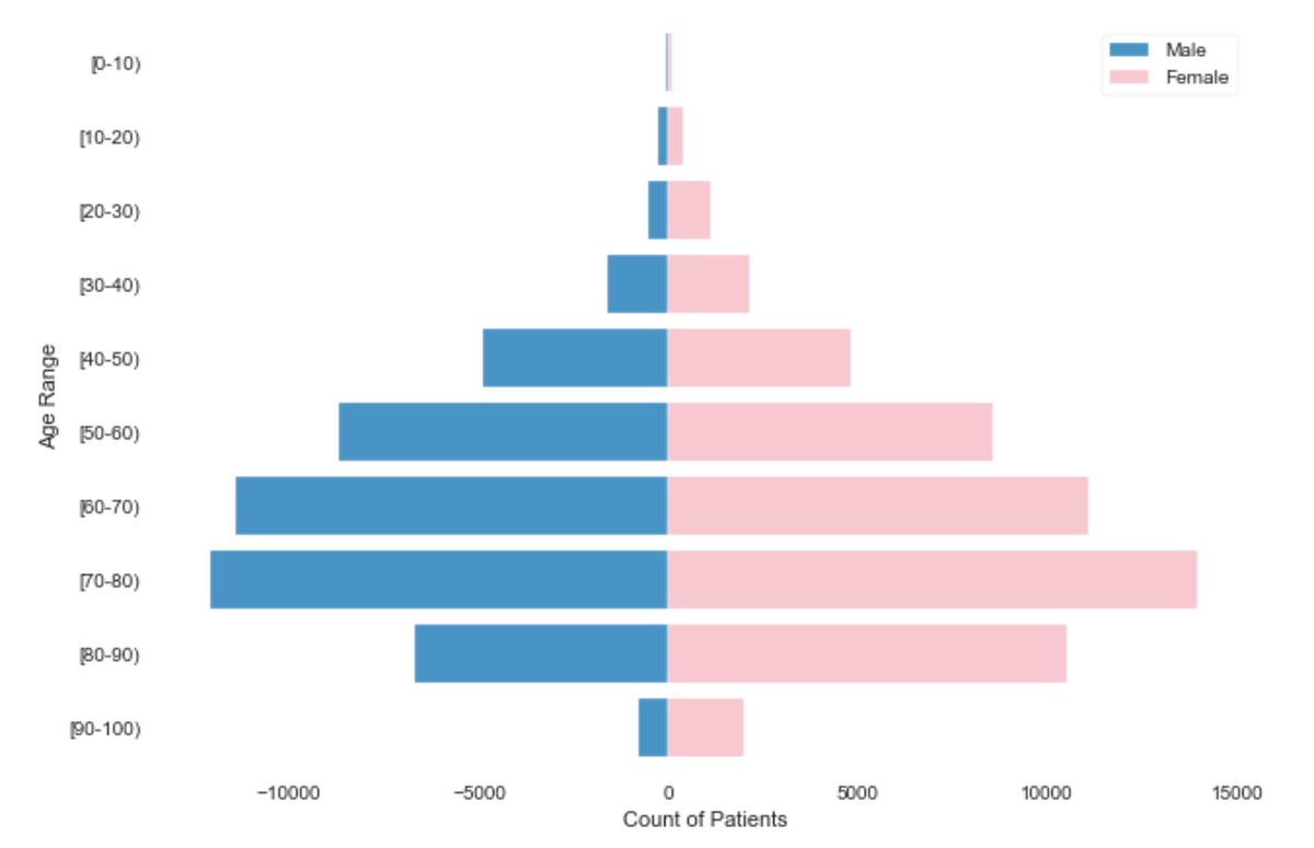
Understanding the distribution of age and gender in our dataset is essential in order to make sure we are reducing the bias between them as much as possible. Studies have discovered that many models are extremely biased, as they’ve only been trained on one gender or race (often men or white people, for example), so this is an extremely important step in the EDA.

Correlations

Often a lot of emphasis in EDA is on correlations, and often correlations are really interesting, but not wholly useful alone (see this article on interpreting basic correlations). A significant area of research in academia is how to identify causation versus correlation (for a brief intro see this Khan Academy lesson), often though domain experts can verify that a correlation is indeed causation.

There are many ways to plot correlations, and different correlation methods to use. I will focus on three —Phi K, Cramer’s V, and ‘one-way analysis’.

Phi K Correlation

Phi_K is a new correlation coefficient based on improvements to Pearson’s test of independence of two variables (see the documentation for more info). See below Phi K correlation from Pandas Profiling (one of several available correlation matrices)

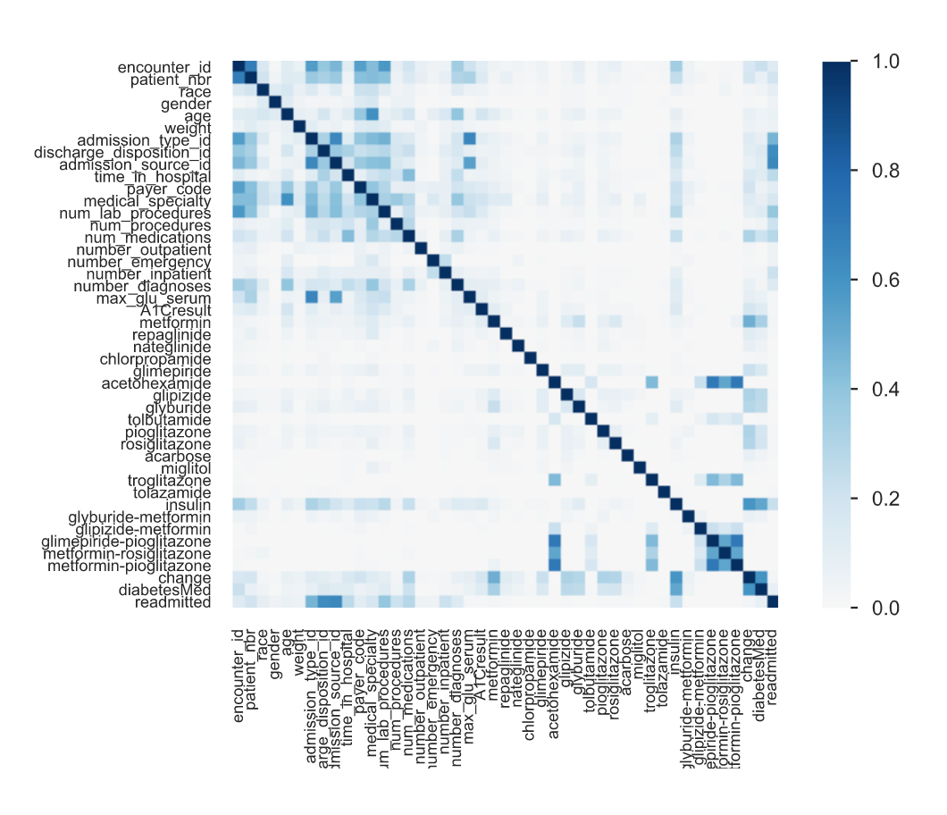
We can very easily identify a correlation between ‘Readmitted’ — our target variable — (the last row/column) and several other features such as: ‘Admission Type’, ‘Discharge Disposition’, ‘Admission Source’, ‘Payer Code’ and ‘Number of Lab Procedures’. This should be light a lightbulb for us, and we must dig deeper into each one to understand if this makes sense in the context of the problem (probably — if you have more procedures then you probably have a more significant problem and so you are more likely to be readmitted), and to help confirm conclusions that our model might find later in the project.

Cramer’s V Correlation

Cramer’s V is a great statistic to measure the correlation between two variables. In general, we are usually interested in the correlation between a feature and the target variable.

Sometimes we can discover other interesting and sometimes surprising information from correlation diagrams, take for example one interesting fact discovered by Lilach Goldshtein in the diabetes dataset. Let us look at the Cramer’s V of ‘discharge_disposition_id’ (a categorical feature that indicates the reason a patient was discharged) and ‘readmitted’ (our target variable — whether or not the patient was readmitted).

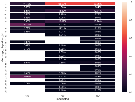
We note here that Discharge ID 11, 19, 20, and 21 have no readmitted patients — STRANGE!

Let’s check what these IDs are:

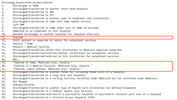
These people were never readmitted because sadly, they passed away.

This is a very obvious note — and we probably didn’t need to dig into data correlations to identify this fact — but such observations are often completely missed. Now a decision needs to be made regarding what to do with these samples — do we include them in the model or not? Probably not, but again that is up to the data scientist. What is important at the EDA stage is that we find these occurrences.

One-Way Analysis

Honestly, if you do one thing I outline in this entire article — do this. One-way analysis can pick up on many of the different observations I’ve touched on in this article, in one graph.

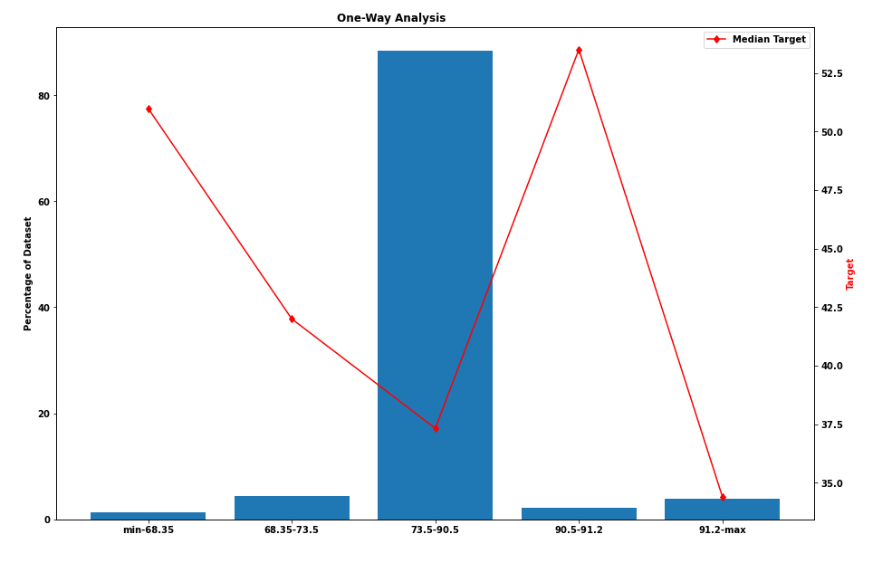
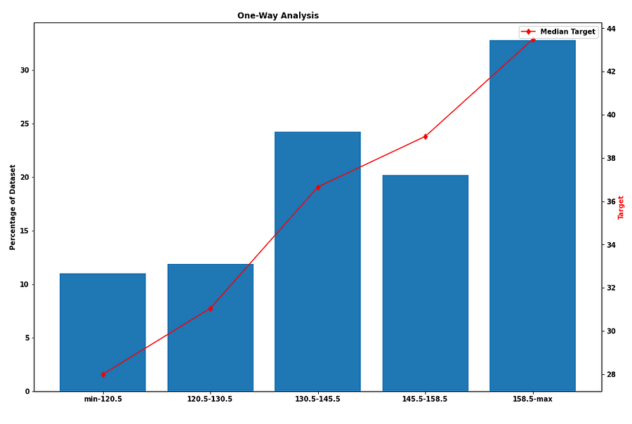
The above graphs show us the percentage of the dataset represented by a certain range and the median of the target variable in that range (this is not the diabetes dataset, but rather a dataset to be used for regression). On the left, we can see that most samples fall in the range 73.5–90.5 and that there is no linear correlation between the feature and the target. On the other hand, on the right-hand side we can see that the feature is directly correlated with the target and that in each group there is a good spread of samples.

The groups were chosen using a single Decision Tree to split optimally.

This is a great way to analyze the dataset. We can see the distribution of the samples in a specific feature, we can see outliers if there are any (none in these examples) and we can identify missing values (either we encode them first as extreme numerical values as described before, or if it is a categorical feature we will see the label as “NaN” or in the diabetes case “?”).

Conclusion

As you have probably noticed by now — there is no one size fits all for EDA. In this article, I decided not to dive too deep into how to do each part of the analysis (most can be done with simple Pandas or Pandas Profiling methods), but rather explain what can we learn from each step and to help those who want to learn why each step is important.

In real-world datasets there are almost always missing values, errors in the data, unbalanced data, and biased data. EDA is the first step in tackling a data science project to learn what data we have and evaluate its validity.

I would like to thank Lilach Goldshtein for her excellent talk on EDA which inspired this medium article.

If you enjoyed this article, be sure to check out — Preparing your Dataset for Modeling and dealing with categorical features — in the next article in the series and the next step in your data journey:

Stay tuned for the next steps in a classic data science project

Part 1 Exploratory Data Analysis (EDA) — Don’t ask how, ask what.

Part 2 Preparing your Dataset for Modelling — Quickly and Easily

Part 3 Feature Engineering — 10X your model’s abilities

Part 4 What is a GBM and how do I tune it?

Part 5 GBM Explainability — What can I actually use SHAP for?

(Hopefully) Part 6 How to actually get a dataset and a sample project