


Drift Detection Using TorchDrift for Tabular and Time-series Data
Last Updated on April 1, 2023 by Editorial Team
Author(s): Rahul Veettil
Originally published on Towards AI.
Learn to monitor your mo in production
Introduction
Machine learning models are designed to make predictions based on data. However, the data in the real world is constantly changing, and this can affect the accuracy of the model. This is known as data drift, and it can lead to incorrect predictions and poor performance. In this blog post, we will discuss how to detect data drift using the Python library TorchDrift.
Table of Contents
- What is Data Drift?
- Types of drifts
- Detecting drift using TorchDrift
- Types of detectors available in TorchDrift
- Maths behind Maximum Mean Discrepancy (MMD) drift
- The dataset used and the computation of statistical differences in the distribution
- TorchDrift on tabular data
- TorchDrift on time series data
- Conclusion
- Link to colab
What is Data Drift?
Data drift occurs when the statistical properties of the data used to train a machine-learning model change over time. This can be due to changes in the input data, changes in the distribution of the input data, or changes in the relationship between the input and output variables. Data drift can cause the model to become less accurate over time, and it is important to detect and correct it to maintain the performance of the model.
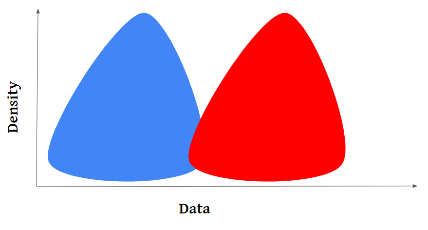
To illustrate the concept, given below are two distributions that are different from each other used in a hypothetical machine learning model, which can result in poor performance issues.
Types of drifts
There are different types of drifts that can occur after the deployment of a machine-learning model. The two prominent ones are:
- Feature drift: The distribution of one or more input variables changes over time. P(X) changes but P(y|X) remains the same.
- Concept drift: The decision boundary change, i.e., P(y/X) changes but P(X) remains the same.
Detecting Model Drift using TorchDrift
Types of Detectors available in TorchDrift
TorchDrift [1] is a PyTorch-based library with several drift detection methods implemented. The 5 different techniques according to the official documentation are given below:
- Drift detector based on (multiple) Kolmogorov-Smirnov tests.
- Drift detector based on the kernel Maximum Mean Discrepancy (MMD) test.
- Implements the kernel MMD two-sample test.
- Computes the p-value for the two-sided two-sample KS test from the D-statistic.
- Computes the two-sample two-sided Kolmorogov-Smirnov statistic.
For more information on the reference papers on which these methods are based, you can have a look at the official documentation.
It seems like this library was originally created to serve image based use-cases (for example: Detecting drifts in production plants or similar applications). Therefore the models are based on pytorch tensors, and the model training is done using Pytorch lightning. It is possible that new users might find it hard to adopt TorchDrift as a library in their use-cases, as they will have to learn both Pytorch and Pytorch lightning to get started. It is also possible that a user is only interested in using the different detectors implemented. Therefore, I intend to show you a tutorial where I will walk you through converting a numpy array into a torch tensor, and focus on making practical usage of the ‘Drift detectors’, without going into other details which are not needed for simple machine learning use-cases.
There are 5 different techniques for detecting model drift within TorchDrift. In this blog post, we will focus on one of the most important detector: The kernel maximum mean discrepancy (MMD) detector.
Maths behind Maximum Mean Discrepancy (MMD) drift
Maximum Mean Discrepancy (MMD) is a statistic that can be used to assert if two distributions P and Q are coming from the same distribution or not. The underlying algorithm in brief is as follows:
- Embed P and Q, the two datasets, in a Hilbert space, where the computation is easier and data is separable.
- Compute the centroids of P and Q in the Hilbert space.
- Measure their distance using the norm.
A Hilbert space helps to generalize from the finite dimensional space to a infinite dimensional space.
The dataset used and the computation of statistical differences in the distribution
TorchDrift on tabular data
The ‘Penguins’ dataset from the seaborn library is selected for performing experiments so that we can focus more on the drift detection part and less on the data itself. The data contains 7 columns with 344 instances each.
As a first step, let’s install the essential libraries and load the data from the seaborn library to examine the data.
pip install torchdrift==0.1.0.post1
pip install seaborn==0.12.2
pip install pandas==1.4.4b
import seaborn as sns
penguins = sns.load_dataset(“penguins”)
penguins.head()
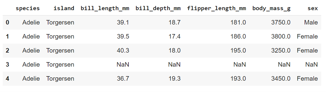
There are 4 numerical attributes, each describing the bill length, bill depth, flipper length, and body mass.
Let’s now have a look at the pairwise correlation between each of these numerical attributes, and what is the difference in their distribution per different classes of penguin species.
sns.set()
sns.pairplot(penguins[[“species”,
“bill_length_mm”,
“bill_depth_mm”,
“flipper_length_mm”,
“body_mass_g”]],
hue = “species”,
size = 2.5)
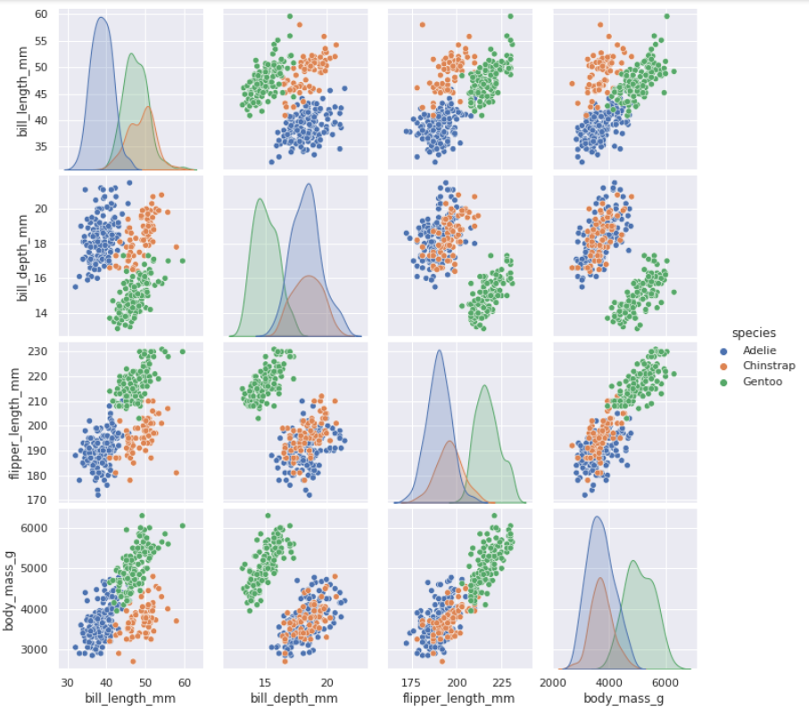
From the above plot, it is very clear that the statistical distribution of the attributes is different for some of the attributes, when subsetted by ‘species’. Let’s write a code to split the data into a train set and test set and look at this difference in distribution more closely for one of these attributes for example ‘flipper_length_mm’.
We will split the data into train-test sets. Note here that, I am splitting the data into train-test tests of 50% each, considering the low number of data records we have. If you plan to build a machine learning model on this dataset, it might be better to split it by Train: 67% and Test: 33%, respectively.
train_set = penguins["flipper_length_mm"][0:172].values
test_set = penguins["flipper_length_mm"][172:].values
Let’s look at the difference in distribution specifically for this attribute.
import pandas as pd
import matplotlib.pyplot as plt
def density_plot(train_set, test_set):
“””Generate a density plot for two 1-D numpy arrays”””
dataset_tensor = pd.DataFrame({‘train_set’ : train_set,
‘test_set’ : test_set},
index=train_set)
dataset_tensor.plot.kde()
plt.xlabel(“Values”, fontsize=22)
plt.ylabel(“Density”, fontsize=22)
density_plot(train_set,test_set)
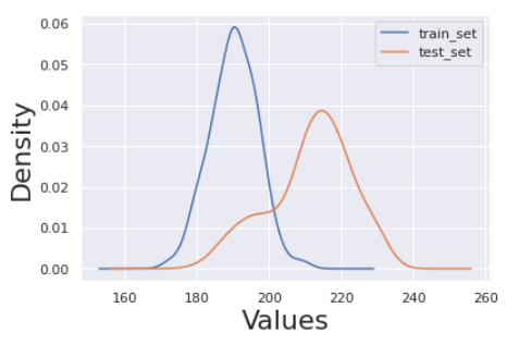
From the above plot, it looks like the train and test sets are different in their statistical distribution. But, how do we know if it is statistically significant? Let’s use TorchDrift to estimate the difference.
We will have to implement 4 functions here :
- numpy_to_tensor — To convert numpy data into a tensor object
- drift_detector — To compute drift
- calculate_drift — To manipulate the data
- plot_driftscore — To plot the output
For the drift detector, we will make use of ‘torchdrift.detectors.KernelMMDDriftDetector’ with the default Gaussian Kernal. We will use a p-value threshold of 0.5 to estimate the significance of the difference in distribution.
import torch
import torchdrift
from torchdrift.detectors.mmd import GaussianKernel
def numpy_to_tensor(trainset, testset):
“”” Convert numpy array to torch tensor”””
train_tensor = torch.from_numpy(trainset)
train_tensor = train_tensor.reshape(trainset.shape[0], 1)
test_tensor = torch.from_numpy(testset)
test_tensor = test_tensor.reshape(testset.shape[0], 1)
return train_tensor, test_tensor
def plot_driftscore(drift_score, train_set, test_set):
“”” Plot drift scores obtained from driftdetector “””
fig = plt.figure(figsize = (25, 10))
gs = fig.add_gridspec(3, hspace=0.5)
axs = gs.subplots(sharex=False, sharey=False)
axs[0].plot(train_set)
axs[0].set_title(“Train data”)
axs[1].plot(test_set)
axs[1].set_title(“Test data”)
axs[2].plot(drift_score, color=’red’,
marker=’o’, linestyle=’dashed’,
linewidth=2, markersize=12)
axs[2].set_title(“p-values”)
def drift_detector(traintensor, testtensor, kernel):
“”” Use torchdrift to calculate p-value for a given test set”””
drift_detector = torchdrift.detectors.KernelMMDDriftDetector(kernel=kernel)
drift_detector.fit(x=traintensor)
p_val = drift_detector.compute_p_value(testtensor)
if p_val < 0.05:
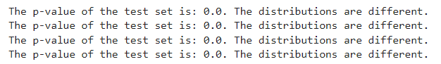
print(f”The test set p-value is: {p_val}. The distributions are different.”)
else:
print(f”The test set p-value is: {p_val}. The distributions are not different.”)
return p_val
def calculate_drift(train_set, test_set, steps=1000,
kernel=”GaussianKernel”):
“”” Calculate drift given a train and test datasets “””
train_set_tensor, test_set_tensor = numpy_to_tensor(train_set, test_set)
drift_score = []
i = 0
while i<len(test_set_tensor):
test_data = test_set_tensor[i:i+steps]
p_value = drift_detector(train_set_tensor, test_data, kernel)
i = i + steps
drift_score.append(p_value)
plot_driftscore(drift_score, train_set, test_set)
Finally, we will make use of the functions we wrote and pass the train set and test sets, in order to estimate the difference in our statistical distribution. The ‘calculate_drift’ function expects a train_set, test_set, steps, and kernel as the parameters.
The ‘steps’ parameter indicates if you want to test the ‘test_set’ data as a whole or in segments against the ‘train_set’. If you want to test the data as a whole then the ‘steps’ needed to be larger than the size of the ‘test_set’. Otherwise, you can choose a smaller size for example 50. This feature is quite useful in case you are working with time series data where you will use segments of the data for comparison rather than the data as a whole.
kernel = GaussianKernel()
calculate_drift(train_set,
 test_set,
 steps=len(test_set) +1,
 kernel= kernel)

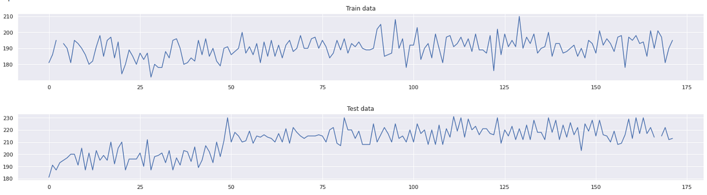
Based on the p-value threshold we set, the computed p-value ie. 0.0 is less than the threshold p-value ie. 0.05, meaning the two datasets are statistically different from each other. You can also observe this difference as a 1-D plot as shown below for both the train and test sets, to understand where the values are drastically changing.
You can change the ‘torchdrift.detectors.KernelMMDDriftDetector’ with any other detector in the ‘drift_detector’ function to test out other types of detectors.
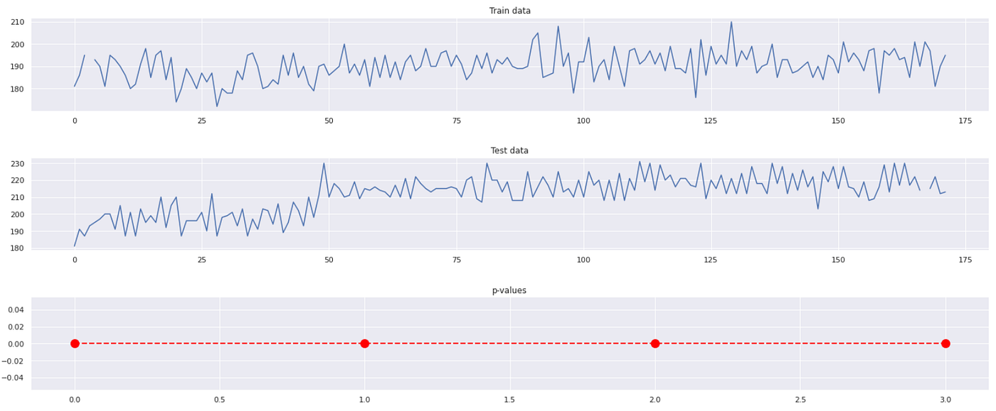
Let’s now use the above function to test the data in segments, with a steps parameter equal to 50. Setting this parameter allows us to test for every 50 points in the ‘test_set’, and to understand how different the considered segment of 50 data points from the ‘train_set’ as a whole.
kernel = GaussianKernel()
compute_drift(train_set,
 test_set,
 steps=50,
 kernel= kernel)
It looks like even when split by segments, for all 4 segments, the ‘test_set’ is statistically different from the train_set. The corresponding plot with p-values for each segment is given below.
TorchDrift on timeseries data
The NYC taxi passengers’ time-series dataset is selected for performing experiments using the same functionalities written above.
import pandas as pd
import numpy as np
taxi_df = pd.read_csv(“https://zenodo.org/record/4276428/files/STUMPY_Basics_Taxi.csv?download=1”)
taxi_df[‘value’] = taxi_df[‘value’].astype(np.float64)
taxi_df.value.plot(figsize = (25, 5))
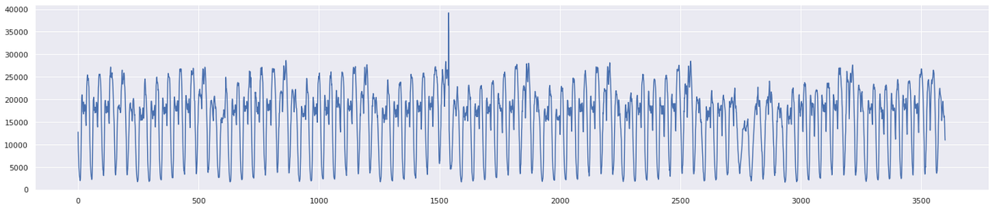
There are 3600 data points each describing the number of passengers in the taxi. I split the data into equal halves for the train and test set, each containing 1800 data points.
train_set = taxi_df.value[0:1800].values
test_set = taxi_df.value[1800:].values
A step size of 300 was used to segment the test data into 6 segments. This allows comparing each segment of 300 test data points to the whole 1800 data points in the train set.
kernel = GaussianKernel()
calculate_drift(train_set,
 test_set,
 steps=300,
 kernel= kernel)
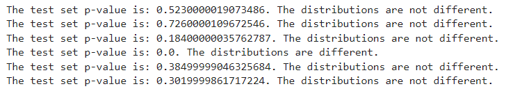
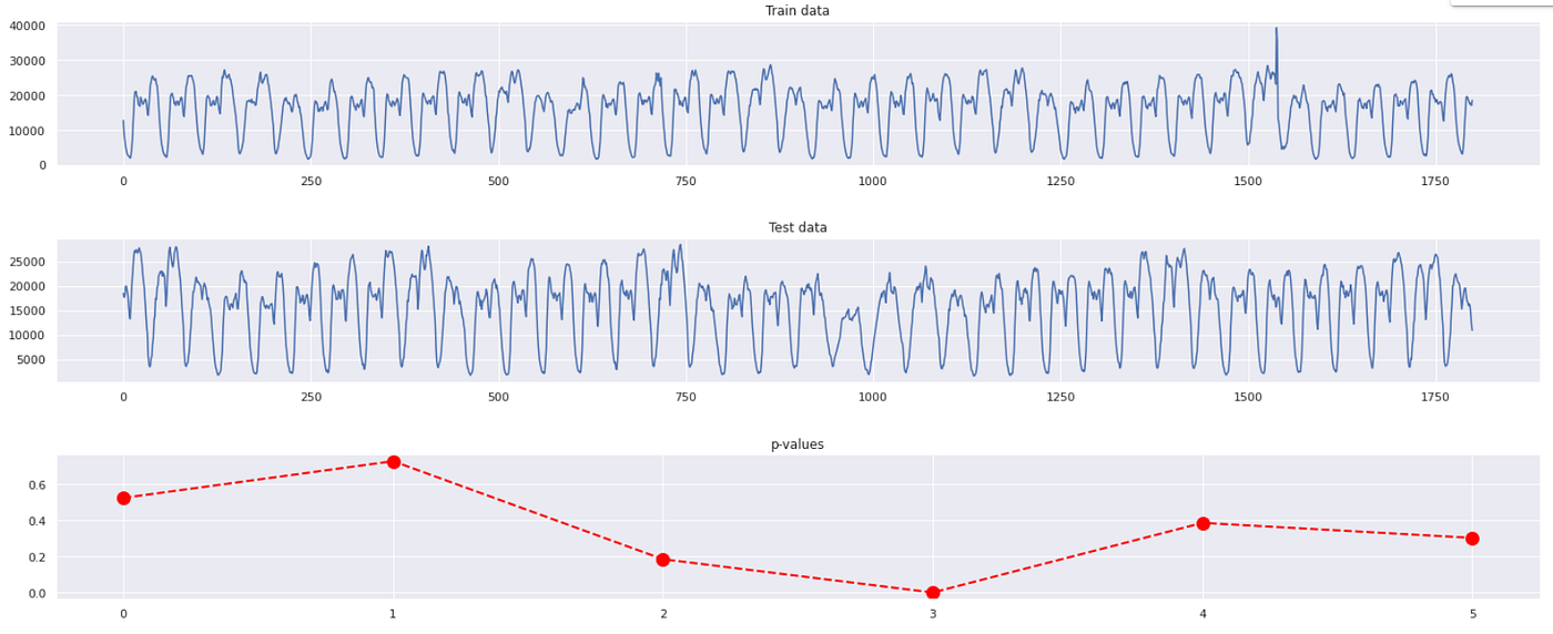
The p-value plot shows that the 4th segment of the data from data points 900 to 1200 in the test set is different from the train set data. If you look at the test data (the 1-D plot in the middle), you will observe that there is a dip in the number of passengers during this period between data points 900 to 1200, validating our finding using TorchDrift. This is quite useful information in case you have an anomaly detection model where you wanted to observe the drift in the number of passengers.
Conclusion
In conclusion, we developed a set of functions to make use of the drift detection algorithm KernelMMDDriftDetector (MMD) implemented in the TorchDrift python library, to test the difference in distribution between two datasets. We tested the functions developed on two datasets namely the tabular dataset of Penguins, and the time series dataset on NYC taxi passengers.
Using the “penguin” dataset, we estimated the statistical distribution between the flipper_length of the birds by splitting the data into equal train and test sets. We estimated the significance of the p-value and found it to be less than 0.05.
Using the NYC taxi passenger dataset, we estimated the statistical distribution of passengers using the taxi for various time periods and identified a decrease in the number of passengers during a time period using a p-value threshold of less than 0.05.
If you are working in a domain where either the data change continuously or you want to test the statistical difference between the train, validation, and test set, you can use the above functions without worrying about the underlying implementation within TorchDrift.
Link to Colab
The complete code can be accessed from here.
If you liked my article, keep watching, I plan to write on several topics in data science, problem-solving, cancer medicine, and psychology for success.
If you would like to connect, please add me on Linkedin.
References
- Thomas Viehmann, Luca Antiga, Daniele Cortinovis, Lisa Lozza, https://torchdrift.org/
Join thousands of data leaders on the AI newsletter. Join over 80,000 subscribers and keep up to date with the latest developments in AI. From research to projects and ideas. If you are building an AI startup, an AI-related product, or a service, we invite you to consider becoming a sponsor.
Published via Towards AI
Towards AI Academy
We Build Enterprise-Grade AI. We'll Teach You to Master It Too.
15 engineers. 100,000+ students. Towards AI Academy teaches what actually survives production.
Start free — no commitment:
→ 6-Day Agentic AI Engineering Email Guide — one practical lesson per day
→ Agents Architecture Cheatsheet — 3 years of architecture decisions in 6 pages
Our courses:
→ AI Engineering Certification — 90+ lessons from project selection to deployed product. The most comprehensive practical LLM course out there.
→ Agent Engineering Course — Hands on with production agent architectures, memory, routing, and eval frameworks — built from real enterprise engagements.
→ AI for Work — Understand, evaluate, and apply AI for complex work tasks.
Note: Article content contains the views of the contributing authors and not Towards AI.
Related posts
Recent Posts


")
