


Diffusion Models vs. GANs vs. VAEs: Comparison of Deep Generative Models
Last Updated on May 16, 2023 by Editorial Team
Author(s): Ainur Gainetdinov
Originally published on Towards AI.
Diffusion Models vs. GANs vs. VAEs: Comparison of Deep Generative Models
Deep generative models are applied to diverse domains such as image, audio, video synthesis, and natural language processing. With the rapid development of deep learning techniques, there has been an explosion of different deep generative models in recent years. This has led to a growing interest in comparing and evaluating these models in terms of their performance and applicability to different domains. In this paper, we aim to provide a comprehensive comparison of deep generative models, including Diffusion Models, Generative Adversarial Networks (GANs), and Variational Autoencoders (VAEs). I will review their underlying principles, strengths, and weaknesses. My goal is to provide a clear understanding of the differences and similarities among these models to guide researchers and practitioners in choosing the most appropriate deep generative model for their specific applications.
Here is a quick summary of how GANs, VAEs, and Diffusion Models models work.
GANs [1, 2] learn to generate new data similar to a training dataset. It consists of two neural networks, a generator, and a discriminator, that play a two-player game. The generator takes in random values sampled from a normal distribution and produces a synthetic sample, while the discriminator tries to distinguish between the real and generated sample. The generator is trained to produce realistic output that can fool the discriminator, while the discriminator is trained to correctly distinguish between the real and generated data. The top row of Figure 1 shows the scheme of its work.
VAEs [3, 4] consist of an encoder and a decoder. The encoder maps high-dimensional input data into a low-dimensional representation, while the decoder attempts to reconstruct the original high-dimensional input data by mapping this representation back to its original form. The encoder outputs the normal distribution of the latent code as a low-dimensional representation by predicting the mean and standard deviation vectors. The middle row of Figure 1 demonstrates its work.
Diffusion models [5, 6] consist of forward diffusion and reverse diffusion processes. Forward diffusion is a Markov chain that gradually adds noise to input data until white noise is obtained. It is not a learnable process and typically takes 1000 steps. The reverse diffusion process aims to reverse the forward process step by step removing the noise to recover the original data. The reverse diffusion process is implemented using a trainable neural network. The bottom row of Figure 1 shows that.
Next, I will outline the key features of different models to help you develop an intuition and make informed decisions when selecting models for your specific use cases.
GANs
- It consists of two neural nets: the generator and the discriminator.
- Training by adversarial loss. The generator aims to “fool” a Discriminator by generating samples that are indistinguishable from real ones. The aim is to make the discriminator unable to differentiate between true and generated samples.
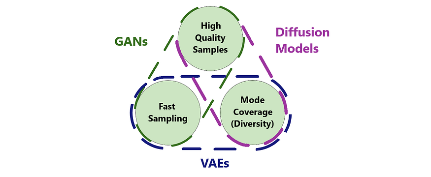
- High-fidelity samples. A neural net is converged, then the discriminator can’t distinguish between real and generated samples. This leads to very realistic samples.
- Low diversity samples. Adversarial loss doesn’t have the incentive to cover the entire data distribution. When the discriminator has overtrained or catastrophic forgetting happens, the generator might be happy enough to produce a small part of the data diversity. This is a common problem and is called mode collapse[2].
- Hard to train. It can be difficult to determine when your network converged. Instead of monitoring one loss going down you should look at two losses that don’t have simple interpretation and sometimes it’s not clear what is happening with your neural net. Offen you need to cope with mode collapse.
- There is a simple trade-off of diversity for fidelity with a truncation trick.
VAEs
- It consists of two neural nets: the encoder and the decoder.
- Training by maximizing log of likelihood, which after mathematical simplifications, becomes L2 loss. It estimates the discrepancy between input and generated samples.
- Low-fidelity samples. There are several reasons:
1. Since the encoder predicts the distribution of the latent code, there may be cases where two distributions of latent codes overlap with each other. Therefore, if two inputs have the same latent code, the optimal decoding would be the average of the two inputs. This leads to blurred samples. Gan and diffusion models do not have this problem.
2. It has a pixel-based loss. The generation of an image with hair will consist of alternating light and dark pixels. If the generation is shifted by only one pixel, the similarity loss with the ground truth would significantly increase or decrease. However, VAEs do not retain such pixel-level information because the latent space is much smaller than the image. This induces the model to predict an average of light and dark pixels to find the optimal solution, resulting in a blurry image. GANs don’t have such a problem because the discriminator can use the blurriness of samples to discriminate between real and generated ones. Similarly, diffusion models, despite having the same pixel-based loss, don’t have this issue. They rely on the current noisy image structure obtained from the ground truth to predict the next step of denoising. - High diversity samples. Likelihood maximization forces to cover all modes of the training dataset, providing neural nets capacity for each train datapoint.
- Easy to train. It has one tractable likelihood loss.
- Encoder enables you to get a latent code of any image, this provides additional possibilities beyond just the generation.
Diffusion Models
- It consists of a fixed forward diffusion process and a learnable reverse diffusion process.
- The forward diffusion process is a multi-step process that gradually adds a small amount of Gaussian noise to the sample until it becomes white noise. A commonly used value for the number of steps is 1000.
- The reverse diffusion process is also a multi-step process that reverses the forward diffusion process, taking the white noise back to an image. Each step of the reverse diffusion process is carried out by a neural network, and it has the same number of steps as the forward process.
- Training by maximizing log of likelihood, which after mathematical simplifications, becomes L2 loss. During training, we calculate noisy images for T and T-1 steps using a formula for a randomly selected T value. The diffusion model then predicts the T-1 step image from the T-step noisy image. The generated image and the T-1 step image are compared using an L2 loss.
- High-fidelity samples. It’s due to the nature of gradually removing noise. Unlike VAEs and GANs, which generate samples at once, diffusion models create samples step by step. The model first creates a coarse image structure and then focuses on adding fine details on top.
- High diversity samples. Likelihood maximization covers all modes of the training dataset.
- The intermediate noisy images serve as latent codes and have the same size as the training images. This is one of the reasons why diffusion models can generate high-fidelity samples.
- Easy to train. It has one tractable likelihood loss.
- Slow sample generation. Unlike GANs and VAEs, it requires multiple runs of the neural net to gradually generate samples. Although there are sampling methods that can accelerate this process by orders of magnitude, they are still much slower than GANs and VAEs.
- The multiple-step process gives new functionalities, such as inpainting or image-to-image generation, simply by exploiting the input noise.
Conclusion
GANs, VAEs, and Diffusion Models are all popular deep-learning generative models that have unique features and are suited to different use cases. Each model has its strengths and weaknesses, and it’s important to understand its nuances before selecting one for a particular application.
I hope this information was helpful to you. Thank you for reading!
References
- Generative Adversarial Nets. Ian J. Goodfellow, Jean Pouget-Abadie, Mehdi Mirza, Bing Xu, David Warde-Farley, Sherjil Ozair, Aaron Courville, Yoshua Bengio — https://arxiv.org/pdf/1406.2661.pdf
- GAN Mode Collapse Explanation — https://medium.com/towards-artificial-intelligence/gan-mode-collapse-explanation-fa5f9124ee73
- Auto-Encoding Variational Bayes. Diederik P Kingma, Max Welling — https://arxiv.org/pdf/1312.6114.pdf
- Understanding Variational Autoencoders (VAEs) — https://towardsdatascience.com/understanding-variational-autoencoders-vaes-f70510919f73
- Deep Unsupervised Learning using Nonequilibrium Thermodynamics. Jascha Sohl-Dickstein, Eric A. Weiss, Niru Maheswaranathan, Surya Ganguli — https://arxiv.org/pdf/1503.03585.pdf
- What are Diffusion Models? Lilian Weng — https://lilianweng.github.io/posts/2021-07-11-diffusion-models
Join thousands of data leaders on the AI newsletter. Join over 80,000 subscribers and keep up to date with the latest developments in AI. From research to projects and ideas. If you are building an AI startup, an AI-related product, or a service, we invite you to consider becoming a sponsor.
Published via Towards AI
Towards AI Academy
We Build Enterprise-Grade AI. We'll Teach You to Master It Too.
15 engineers. 100,000+ students. Towards AI Academy teaches what actually survives production.
Start free — no commitment:
→ 6-Day Agentic AI Engineering Email Guide — one practical lesson per day
→ Agents Architecture Cheatsheet — 3 years of architecture decisions in 6 pages
Our courses:
→ AI Engineering Certification — 90+ lessons from project selection to deployed product. The most comprehensive practical LLM course out there.
→ Agent Engineering Course — Hands on with production agent architectures, memory, routing, and eval frameworks — built from real enterprise engagements.
→ AI for Work — Understand, evaluate, and apply AI for complex work tasks.
Note: Article content contains the views of the contributing authors and not Towards AI.
Related posts
Recent Posts
")


")


