


Clustering unveiled: The Intersection of Data Mining, Unsupervised Learning, and Machine Learning
Last Updated on January 25, 2024 by Editorial Team
Author(s): Anand Raj
Originally published on Towards AI.
Table of Contents
- Introduction
- K- Means Clustering Technique
– Metrics for Clustering
– K-means algorithm
– Lloyd’s algorithm (approximation approach)
– Initialization Sensitivity
– K-means++ Initialization
– Limitations of K-means
– K-medoids with PAM algorithm
– Determining the right K
– Time and Space Complexity - Hierarchical Clustering Technique
– Agglomerative Hierarchical Clustering
– Proximity methods
– Time and Space Complexity
– Advantages and Limitations - DBSCAN Clustering Technique
– DBSCAN algorithm
– Determining the hyperparameters
– Advantages and Limitations - Applications
- References
Introduction
Clustering is a topic that can be associated with both Data Mining and Machine Learning. Clustering involves grouping similar data points together based on certain features or characteristics. In the context of Data Mining, clustering is often used as a technique to discover patterns, structures, or relationships within a dataset. It can help identify natural groupings or clusters in the data, which may have inherent meaning or significance. In the realm of Machine Learning, clustering is considered a type of unsupervised learning. Unsupervised learning involves exploring and analyzing data without labeled outputs or target variables. Clustering algorithms are used to automatically identify patterns or groupings in the data without any predefined categories. In summary, clustering is a technique that can be applied in both the Data Mining and Machine Learning domains, and it plays a significant role in tasks related to pattern discovery, data exploration, and unsupervised learning.
1. K- Means Clustering Technique
Metrics for Clustering
Before delving into the diverse clustering algorithms, it’s essential to comprehend the metrics associated with clustering. This understanding will provide a stronger foundation for exploring the intricacies of clustering methods.
Mathematical Representation
The Dunn index is often expressed mathematically as the ratio of the minimum inter-cluster distance to the maximum intra-cluster distance. Here’s a more detailed representation:
Let dinter(Ci,Cj) be the distance between clusters Ci and Cj, and dintra(Ck) be the distance within cluster Ck. Where, k is number of clusters.
The mathematical formula for the Dunn index (D) is given by:

In simpler terms, the Dunn index compares the smallest distance between different clusters to the largest distance within any single cluster. A higher Dunn index suggests better-defined and more separated clusters, indicating a potentially better clustering solution.
Geometrical representation

Here, is the simple geometric representation with two clusters C1(data points — yellow stars) and C2 (data points — blue stars) plotted across feature 1(F1) and feature 2(F2). Where the red line depicts the nearest distance between data point in cluster C1 and cluster C2(inter-cluster distance). Blue and yellow lines depict the farthest distance between the points within the cluster C1 and cluster C2, respectively. The ratios of these values helps us determine Dunn Index.
There are many other metrics available but the core idea is remains the same, as mentioned below:
- Lower intra-cluster distance.
- Higher inter-cluster distance.
K-means algorithm
The K-Means algorithm minimizes an objective function that represents the sum of squared distances between data points and their assigned cluster centroids. The goal is to find cluster assignments and centroid positions that minimize this overall distance. Let’s delve into the mathematical formulation of the K-Means objective function:
Objective Function (Sum of Squared Distances):

The goal of the K-Means algorithm is to find cluster assignments ci and centroid positions μk that minimize the objective function J. The mathematical formulation of the K-Means objective function is NP-hard to solve due to the combinatorial nature of exploring all possible assignments of data points to clusters, making an exhaustive search computationally infeasible. Iterative algorithms like Lloyd’s offer a pragmatic approach by iteratively refining cluster assignments and centroids, providing a computationally efficient approximation to the optimal solution.
Lloyd’s algorithm (approximation approach)
Lloyd’s algorithm, also known as the K-Means algorithm, is an iterative optimization approach for clustering that aims to minimize the K-Means objective function. It serves as an approximation method to find a locally optimal solution for the NP-hard K-Means problem. Here’s an elaboration on the key steps of Lloyd’s algorithm:
1. Initialization:
- Randomly select K initial centroids from the dataset.
2. Iterative Assignment and Update:
a. Assignment Step:
- Assign each data point to the nearest centroid based on Euclidean distance.

b. Update Step:
- Recalculate the centroids based on the mean of the data points assigned to each cluster.

3. Convergence:
- Repeat the assignment and update steps until convergence, typically when there is little or no change in cluster assignments or centroid positions between iterations.
Lloyd’s algorithm is sensitive to the initial placement of centroids and may converge to a local minimum of the objective function. Therefore, it is common to run the algorithm multiple times with different initializations and choose the solution with the lowest objective value.
Lloyd’s algorithm provides a practical and computationally efficient solution to the K-Means clustering problem. By iteratively updating cluster assignments and centroids, it converges to a locally optimal solution. Its simplicity, efficiency, and scalability make it a widely adopted algorithm for clustering tasks in various fields, despite the challenges associated with local optima.
Initialization Sensitivity
Lloyd’s algorithm is susceptible to convergence to local minima, and the quality of the solution depends on the initial centroid positions. Hence, suffers from initialization sensitivity. Thus, we introduce K-means++ technique to tackle this problem.
We can understand from the below geometric representations the importance of choosing initial centroids and slight variation in them can result in different K-means clustering.


To mitigate sensitivity to initial centroid selection in K-Means we employ K-Means++ with a smarter initialization scheme, reducing the risk of converging to suboptimal solutions and enhancing the algorithm’s overall performance. The probabilistic selection of initial centroids in K-Means++ promotes a more representative and diverse set, leading to improved clustering results.
K-means++ Initialization
The K-Means++ initialization technique aims to improve the convergence and final quality of clusters in the K-Means algorithm by selecting initial centroids more strategically. The key steps of K-Means++ are as follows:
- Initialization:
- The first centroid is randomly selected from the data points.
2. Probabilistic Selection:
- Subsequent centroids are chosen with a probability proportional to the square of the Euclidean distance from the point to the nearest existing centroid.
- This probabilistic approach ensures that new centroids are placed at a considerable distance from each other, promoting a more even spread across the dataset.
3. Repeat Until K Centroids are Chosen:
- Steps 1 and 2 are repeated until K centroids are selected.
4. K-Means Algorithm with K-Means++ Initialization:
- The selected centroids are then used as the initial centroids in the standard K-Means algorithm.
The benefits of K-Means++ include a reduction in the number of iterations required for convergence and an improved likelihood of finding a better global optimum. This initialization scheme is particularly effective in addressing the sensitivity of K-Means to the initial placement of centroids, resulting in more stable and representative clustering outcomes.
Limitations of K-means
- K-Means tend to produce clusters of approximately equal sizes, which may not be suitable for datasets with unevenly distributed or hierarchical structures.

- K-Means assumes that clusters have similar densities, which may not hold in cases where clusters have varying densities. It may struggle to adapt to clusters with regions of varying data point concentration.

- K-Means assumes clusters to be spherical. If clusters have non-globular shapes, such as elongated structures or irregular geometries, K-Means may fail to represent the underlying structure accurately, leading to suboptimal results.

- K-Means is sensitive to outliers, as it minimizes the sum of squared distances. Outliers can disproportionately influence the centroid positions, leading to clusters that are skewed or misplaced.
- The centroids generated by K-Means may not have clear and meaningful interpretations, especially in high-dimensional spaces or when dealing with complex, heterogeneous data. Each centroid is a point in the feature space but may not correspond to a recognizable or easily interpretable data point. This can be overcome by K-Medoids clustering technique explained in the next section.
One solution to overcome these limitations, is to use many clusters. Find parts of clusters, but the major task here is we need to put these smaller parts of clusters together, to achieve optimal clusters as per original points.

K-medoids with PAM algorithm
The K-Medoids technique uses an algorithm called the PAM algorithm (Partitioning Around Medoids). The PAM algorithm is a partitional clustering algorithm, similar to K-Means, but it focuses on selecting representative points (data points) in each cluster known as “medoids” instead of centroids.

Here’s an overview of how the PAM algorithm works in the context of K-Medoids:
- Initialization:
- Initially, K data points are selected as the medoids.
2. Assignment:
- Each data point is assigned to the closest medoid based on a chosen distance metric (commonly using measures like Euclidean distance).
3. Update:
- For each cluster, the data point that minimizes the sum of distances to all other points in the cluster is selected as the new medoid.
4. Iteration:
- Steps 2 and 3 are iteratively repeated until there is minimal or no change in the assignment of points to clusters and the selection of medoids.
5. Final Clusters:
- The final clusters are determined by the data points assigned to the medoids.
The PAM algorithm is more robust to outliers compared to K-Means, as it directly chooses medoids as representatives, which are less influenced by extreme values. It is especially suitable for situations where the mean (used in K-Means) may not be a meaningful representative, and the medoid provides a more interpretable and robust choice.
K-Medoids, utilizing the PAM algorithm, is commonly used in situations where the interpretability of clusters and robustness to outliers are crucial considerations. In addition, it also has an advantage of kernelization over K-means.
Determining the right K
The Elbow Method is a popular technique for determining the optimal number of clusters (K) in a dataset when using clustering algorithms like K-Means or K-Medoids. The idea behind the method is to observe the relationship between the number of clusters and the within-cluster sum of squared distances (inertia or error). The “elbow” in the plot represents a point where increasing the number of clusters ceases to result in a significant reduction in the sum of squared distances.
Here’s an illustrative interpretation of an Elbow Method plot. In the example, the elbow point is at K = 3, suggesting that three clusters are a reasonable choice for the given dataset.

Time and Space Complexity
1. Time Complexity:
- O(I * K * n * d), where I is the number of iterations, K is the number of clusters, n is the number of data points, and d is the number of dimensions.
2. Space Complexity:
- O(n * d), where n is the number of data points and d is the number of dimensions.
Hence, both time and space complexity are linear for the K-means technique and its variants (K-means++, K-medoids).
2. Hierarchical Clustering Technique
Hierarchical clustering is a technique used in unsupervised machine learning to group similar data points into clusters in a hierarchical structure. The key feature of hierarchical clustering is that it creates a tree-like structure, called a dendrogram, which visually represents the relationships and structures within the data.
There are two main types of hierarchical clustering: agglomerative and divisive.
Agglomerative hierarchical clustering starts with individual data points as separate clusters and iteratively merges the most similar clusters, forming a hierarchical structure. In contrast, divisive hierarchical clustering begins with all data points in a single cluster and progressively divides the least similar clusters, generating a hierarchical tree that represents the relationships within the dataset. Both methods create dendrograms for visualizing clustering structures.
Agglomerative Hierarchical Clustering
The more popular hierarchical clustering technique is Agglomerative Clustering. Agglomerative Hierarchical Clustering algorithm is a bottom-up approach that starts with individual data points as separate clusters and progressively merges them based on their proximity matrix. The process continues until all data points belong to a single cluster. Here is a step-by-step explanation of the agglomerative hierarchical clustering algorithm:
- Initialization:
- Treat each data point as a singleton cluster. Initially, there are N clusters for N data points.
2. Compute the proximity matrix:
- Calculate the proximity (distance) between each pair of clusters.

3. Find Closest Pair of Clusters:
- Identify the pair of clusters with the smallest proximity. This pair will be merged in the next step.
4. Merge Closest Clusters:
- Combine (merge) the two clusters identified in step 3 into a new cluster. The proximity matrix is updated to reflect the distances between the new cluster and the remaining clusters.


5. Repeat Steps 2 to 4:
- Iterate steps 2 to 4 until only a single cluster remains, capturing the hierarchical structure of the data.
6. Dendrogram Construction:
- Construct a dendrogram to visualize the hierarchy of cluster mergers. The height at which two branches merge in the dendrogram represents the proximity at which the corresponding clusters were combined.

7. Cutting the Dendrogram:
- Determine the number of clusters by “cutting” the dendrogram at a certain height. The height at the cut represents the proximity threshold for forming clusters.
Proximity methods
In Agglomerative Hierarchical Clustering, proximity methods refer to the metrics used to calculate the dissimilarity or similarity (proximity) between clusters. These methods play a crucial role in determining how clusters are merged during the agglomeration process. Common proximity methods include:
MIN method / Single Linkage (Nearest Neighbor):
- The proximity between two clusters is defined as the minimum distance between any pair of points, one from each cluster. It is sensitive to outliers and tends to form elongated clusters.


MAX method / Complete Linkage (Farthest Neighbor):
- The proximity between two clusters is defined as the maximum distance between any pair of points, one from each cluster. It is less sensitive to outliers than single linkage and tends to form more compact clusters.


Group Average method / Average Linkage:
- The proximity between two clusters is defined as the average distance between all pairs of points, one from each cluster. It balances sensitivity to outliers and tends to produce clusters of moderate compactness.


Centroid Linkage:
- The proximity between two clusters is defined as the distance between their centroids (means). It can be less sensitive to outliers than single linkage but may lead to non-compact clusters.

Ward’s linkage:
- Ward’s linkage, a proximity method in Agglomerative Hierarchical Clustering, minimizes the increase in variance within merged clusters. It tends to form compact and evenly sized clusters, making it less sensitive to outliers than some other linkage methods. Similar to group average with distance between points is a squared distance.

Time and Space Complexity
The time and space complexity of hierarchical clustering algorithms depends on several factors including the number of data points (N), the dimensionality of the data (D), and the specific implementation of the algorithm.
Time Complexity:
- The time complexity is often in the range of O(N² log N) to O(N³). The dominant factor is the computation of pairwise distances between clusters, which requires O(N²) operations in each iteration. The logarithmic factor accounts for the hierarchical structure.
Space Complexity:
- The space complexity is usually O(N²) for storing the dissimilarity matrix between clusters. Additional memory may be required for storing the hierarchical tree structure (dendrogram).
Advantages and Limitations
Advantages of Hierarchical Clustering:
- Hierarchical Structure Representation:
- Provides a natural and intuitive representation of the hierarchical relationships within the data through dendrograms, allowing for a clear visualization of clusters at different scales.
2. No Predefined Number of Clusters:
- Does not require specifying the number of clusters in advance, making it suitable for datasets where the number of clusters is not known beforehand.
3. Flexibility in Interpretation:
- Offers flexibility in interpreting clustering results at different levels of granularity, allowing users to explore the data structure at various resolutions.
Limitations of Hierarchical Clustering:
- Computational Complexity in time and space:
- Hierarchical clustering’s computational cost increases with large datasets due to proximity matrix calculations and dendrogram updates, posing challenges in memory storage for extensive datasets.
2. Sensitivity to Noise and Outliers:
- Sensitive to noise and outliers, particularly in agglomerative clustering methods that may merge clusters based on proximity, leading to distorted clusters.
3. No objective function is directly minimized.
- Hierarchical clustering lacks a direct objective function to minimize during the clustering process, making it challenging to quantitatively assess the quality of clustering results and compare different hierarchical structures objectively.
3. DBSCAN Clustering Technique
DBSCAN (Density-Based Spatial Clustering of Applications with Noise) is a clustering algorithm designed to identify clusters of arbitrary shapes in a dataset, while also marking data points that do not belong to any cluster as noise.
Here’s an elaboration on DBSCAN:
- Density-Based Clustering:
- DBSCAN operates based on the concept of density, defining clusters as dense regions separated by sparser areas. It doesn’t assume a spherical cluster shape and can identify clusters of varying shapes and sizes.
2. Parameter:
- DBSCAN requires two parameters: the radius (ε) that defines the neighborhood around a point, and the minimum number of points (MinPts) within that radius to consider a point a core point.
3. Core Points, Border Points, and Noise:
- DBSCAN classifies data points into three categories: core points, which have a sufficient number of neighboring points within a specified radius; border points, which are within the radius of a core point but do not have enough neighbors themselves; and noise points, which have insufficient neighbors and do not belong to any cluster.


4. Density-Reachable (Density Edge) Points:
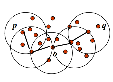
- A point P is density-reachable from another point Q with respect to parameters ε (radius) and MinPts (minimum number of points), if there exists a chain of points P1,P2,…,Pn where P1=Q and Pn=P, such that each Pi+1 is directly density-connected to Pi, and the distance between consecutive points is within ε. That is, if Q and P are core points and distance QO is less than or equal to ε then QP forms a density edge.

5. Density-Connected Points:
- Two points P and Q are density-connected with respect to parameters ε and MinPts if there exists a point O such that both P and Q are density-reachable from O. In other words, they are part of the same cluster or connected by a chain of density-reachable points.
DBSCAN algorithm
DBSCAN (Density-Based Spatial Clustering of Applications with Noise) is a clustering algorithm designed to discover clusters of arbitrary shapes in a dataset based on the density of data points. Let’s delve into the details of the DBSCAN algorithm:
- Initialization:
- Choose two parameters: ε (radius) and MinPts (minimum number of points) required to form a dense region. These parameters guide the algorithm’s sensitivity to density.
2. Point Classification:
- For each data point in the dataset, determine whether it is a core point, a border point, or a noise point:
- Core Point: Has at least MinPts data points, including itself, within a distance of ε.
- Border Point: Has fewer than MinPts data points within ε, but is density-reachable from a core point.
- Noise Point: Does not meet the criteria for core or border points.
3. Cluster Formation:
- Form clusters by connecting core points and their density-reachable neighbors. Each core point starts a new cluster, and any density-reachable point becomes part of the cluster. The process continues until no more density-reachable points can be added to the cluster.
4. Border Point Assignment:
- Assign border points to the cluster of their density-reachable core point.
5. Noise Points:
- Mark noise points that are neither core points nor density-reachable from any core point.
The steps of DBSCAN are executed until all points have been classified. The algorithm results in clusters of varying shapes and sizes, and it identifies noise points that do not belong to any cluster.
Determining the hyperparameters
Rule of Thumb for MinPts:
- A common rule of thumb is to set MinPts to roughly twice the dimensionality of the dataset. For example, in a two-dimensional space, MinPts might be set to 4. This provides a balance between sensitivity to local density and avoiding overfitting.
Knee Point Detection (elbow method) for Eps (ε):
- Look for a “knee point” in the k-distance plot, which signifies a transition from dense to sparse regions. This can help determine a suitable ε.

Advantages and Limitations
Advantages of DBSCAN technique:
- Robust to Noise:
- DBSCAN is robust to outliers and noise, as it classifies points that do not fit into dense regions as noise.
2. Handles Arbitrary Cluster Shapes:
- The algorithm can identify clusters with arbitrary shapes and is not limited to predefined geometries.
3. Automatic Cluster Number Determination:
- DBSCAN does not require specifying the number of clusters in advance, adapting to the inherent density structure of the data.

Limitations of DBSCAN technique:
- Sensitive to Parameters:
- The performance of DBSCAN can be sensitive to the choice of ε and Min Pts parameters.
2. Difficulty with Varying Density:
- Struggles with datasets where clusters have varying densities, as a single ε may not suit all regions.
3. Difficulty with High-Dimensional Data:
- The curse of dimensionality can impact the effectiveness of distance-based measures in high-dimensional spaces.

Time and Space complexity
The time and space complexity of DBSCAN (Density-Based Spatial Clustering of Applications with Noise) depend on several factors, including the implementation details, the size of the dataset, and the chosen data structures.
Time Complexity:
- In the worst-case scenario, the time complexity of DBSCAN is often considered to be around O(n²), where n is the number of data points. This is because, in the worst case, each data point needs to be compared with every other data point to determine density-reachability.
Space Complexity:
- The space complexity of DBSCAN is typically O(n), where n is the number of data points. This is mainly due to the storage of the dataset itself and additional structures like the cluster assignments.
4. Applications
Clustering finds diverse applications across industries. In marketing, it aids target audience segmentation; in biology, it helps classify species based on genetic similarities. E-commerce platforms employ clustering for customer behavior analysis, enhancing personalized recommendations. In healthcare, it supports disease profiling for tailored treatments. Clustering is a versatile tool, fostering insights and efficiency.
Have a look through the links provided in the reference section for detailed information.
References
AgglomerativeClustering Code samples
— — — — — — — — — — — — — — — — — — — — — — — — — — — — — — — — — — — — — —
Hope you liked the article!!!!
You may reach out to me on LinkedIn.
Join thousands of data leaders on the AI newsletter. Join over 80,000 subscribers and keep up to date with the latest developments in AI. From research to projects and ideas. If you are building an AI startup, an AI-related product, or a service, we invite you to consider becoming a sponsor.
Published via Towards AI
Take our 90+ lesson From Beginner to Advanced LLM Developer Certification: From choosing a project to deploying a working product this is the most comprehensive and practical LLM course out there!
Towards AI has published Building LLMs for Production—our 470+ page guide to mastering LLMs with practical projects and expert insights!

Discover Your Dream AI Career at Towards AI Jobs
Towards AI has built a jobs board tailored specifically to Machine Learning and Data Science Jobs and Skills. Our software searches for live AI jobs each hour, labels and categorises them and makes them easily searchable. Explore over 40,000 live jobs today with Towards AI Jobs!
Note: Content contains the views of the contributing authors and not Towards AI.
Related posts


Popular posts

 for 2021")


Updates

Recent Posts


