Closed-form and Gradient Descent Regression Explained with Python

Last Updated on January 6, 2023 by Editorial Team

Last Updated on August 7, 2020 by Editorial Team

Author(s): Satsawat Natakarnkitkul

Machine learning, Programming

Regression problem simplified and implementation in Python

Introduction

Regression is a kind of supervised learning algorithm within machine learning. It is an approach to model the relationship between the dependent variable (or target, responses), y, and explanatory variables (or inputs, predictors), X. Its objective is to predict a quantity of the target variable, for example; predicting the stock price, which differs from classification problem, where we want to predict the label of target, for example; predicting the direction of stock (up or down).

Moreover, a regression can be used to answer whether and how several variables are related, or influence each other, for example; determine if and to what extent the work experience or age impacts salaries.

In this article, I will focus mainly on linear regression and its approaches.

Different approaches to Linear Regression

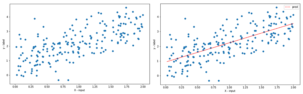
OLS (Ordinary least squares) goal is to find the best-fitting line (hyperplane) that minimizes the vertical offsets, which can be mean squared error (MSE) or other error metrics (MAE, RMSE) between the target variable and the predicted output.

We can implement a linear regression model using the following approaches:

1. Solving model parameters (closed-form equations)
2. Using optimization algorithm (gradient descent, stochastic gradient, etc.)

Please note that OLS regression estimates are the best linear unbiased estimator (BLUE, in short). Regression in other forms, the parameter estimates may be biased, for example; ridge regression is sometimes used to reduce the variance of estimates when there is collinearity in the data. However, the discussion of bias and variance is not in the scope of this article (please refer to this great article related to bias and variance).

Closed-form equation

Let’s assume we have inputs of X size n and a target variable, we can write the following equation to represent the linear regression model.

The equation is assumed we have the intercept X0 = 1. There is also a model without intercept, where B0 = 0, but this is based on some hypothesis that it will always undergo through the origin (there’s a lot of discussion on this topic which you can read more here and here).

From the equation above, we can compute the regression parameters based on the below computation.

Now, let’s implement this in Python, there are three ways we can do this; manual matrix multiplication, statsmodels library, and sklearn library.

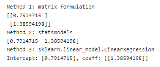
You can see that all three solutions give out the same results, we can then use the output to write the model equation (Y =0.7914715+1.38594198X).

This approach offers a better solution for smaller data, easy, and quick explainable model.

Gradient Descent

Why we need gradient descent if the closed-form equation can solve the regression problem. There will be some situations which are;

• There is no closed-form solution for most nonlinear regression problems.
• Even in linear regression, there may be some cases where it is impractical to use the formula. An example is when X is a very large, sparse matrix. The solution will be too expensive to compute.

Gradient descent is a computationally cheaper (faster) option to find the solution.

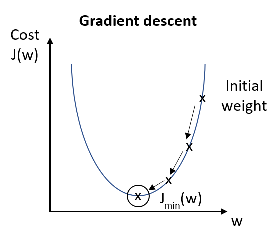
Gradient descent is an optimization algorithm used to minimize some cost function by repetitively moving in the direction of steepest descent. Hence, the model weights are updated after each epoch.

There are three primary types of gradient descent used in machine learning algorithm;

1. Batch gradient descent
2. Stochastic gradient descent
3. Mini-batch gradient descent

Let us go through each type in more detail and implementation.

Batch Gradient Descent

This approach is the most straightforward. It calculates the error for each observation within the training set. It will update the model parameters after all training observations are evaluated. This process can be called a training epoch.

The main advantages of this approach are computationally efficient and producing a stable error gradient and stable convergence, however, it requires the entire training set in memory, also the stable error gradient can sometimes result in the not-the-best model (converge to local minimum trap, instead attempt to find the best global minimum).

Let’s observe the python implementation of the regression problem.

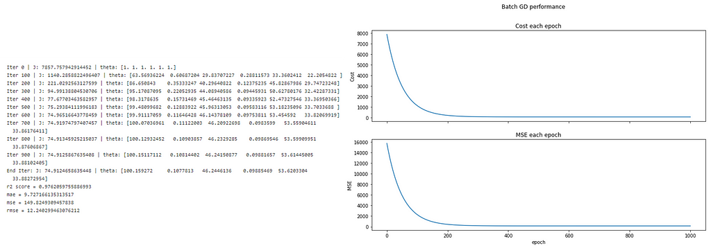
As we can see, the cost is reducing stably and reach a minimum of around 150–200 epochs.

During the computation, we also use vectorization for better performance. However, if the training set is very large, the performance will be slower.

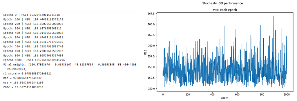
Stochastic Gradient Descent

In stochastic gradient descent, SGD (or sometimes referred to as iterative or online GD). The name “stochastic” and “online GD” come from the fact that the gradient-based on single training observation is a “stochastic approximation” of the true cost gradient. However, because of this, the path towards the global cost minimum is not direct and may go up-and-down before converging to the global cost minimum.

Hence;

• This makes SGD faster than batch GD (in most cases).
• We can view the insight and rate of improvement of the model in real-time.
• Increased model update frequency can result in faster learning.
• Noisy update of stochastic nature can help to avoid the local minimum.

However, some disadvantages are;

• Due to update frequency, this can be more computation expensive, which can take a longer time to complete than another approach.
• The frequent updates will result in a noisy gradient signal, which causes the model parameters and error to jump around, higher variance over training epochs.

Let’s look at how we can implement this in Python.

Mini-Batch Gradient Descent

Mini-batch gradient descent (MB-GD) is a more preferred method since it compromises between Batch gradient descent and stochastic gradient descent. It separates the training set into small batches and feeds to the algorithm. The model will get updates based on these batches. The model will converge more quickly than batch GD because the weights get updated more frequently.

This method combines the efficiency of batch GD and the robustness of stochastic GD. One (small) downside is this method introduces a new parameter “batch size”, which may require the fine-tuning as part of model tuning/optimization.

We can imagine batch size as a slider on the learning process.

• Small value gives a learning process converges quickly at the cost of noise in the training process
• Large value gives a learning process converges slowly with accurate estimates of the error gradient

We can reuse the above function but need to specify the batch size to be len(training set) > batch_size > 1.

theta, _, mse_ = _sgd_regressor(X_, y, learning_rate=learning_rate, n_epochs=n_epochs, batch_size=50)

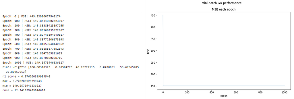
We can see that only the first few epoch, the model is able to converge immediately.

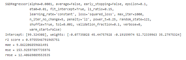
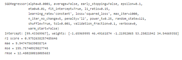
SGD Regressor (scikit-learn)

In python, we can implement a gradient descent approach on regression problem by using sklearn.linear_model.SGDRegressor . Please refer to the documentation for more details.

Below is how we can implement a stochastic and mini-batch gradient descent method.

EndNote

In this post, I have provided the explanation of linear regression on both closed-form equation and optimization algorithm, gradient descent, by implementing them from scratch and using a built-in library.

Additional reading and Github repository:

• 5.4 – A Matrix Formulation of the Multiple Regression Model
• Practical recommendations for gradient-based training of deep architectures
• netsatsawat/close-form-and-gradient-descent-regression-explained

---

Closed-form and Gradient Descent Regression Explained with Python was originally published in Towards AI — Multidisciplinary Science Journal on Medium, where people are continuing the conversation by highlighting and responding to this story.

Published via Towards AI