


A More Intuitive Way To Understand Graph Neural Networks With a Code Example
Last Updated on January 5, 2024 by Editorial Team
Author(s): Ruite Xiang
Originally published on Towards AI.
Sometimes, it is difficult to understand the theory — the math and the formulas- without seeing how it translates into code.
At least, that is my case, so I put together this post to explain the different concepts in graph neural networks (GNNs) in a way that is more intuitive and beginner-friendly, complemented with a code example.
However, when I say beginners, you might still need to know some concepts such as matrix multiplications and Pytorch.
What is a graph?
Graphs are used to represent a set of connected objects, modeled as nodes connected via edges that represent their relationships. Each node is described with a feature vector, which is what the GNNs will use to make the predictions.

For each graph with a set of nodes and edges, we would have a feature matrix (X) and information about how the different nodes are connected.

The connectivity data can be represented in different formats such as an adjacency matrix where 1s represent connections and the row or column index is the edge index.
In the case of PyTorch Geometric, connectivity is represented in the sparse COO format of shape [2, num_edges] with row 0 being the source nodes and row 1 the destination nodes, as you can see in the image.
It is quite a flexible representation since any data where the relationships between the objects are relevant to the prediction task can benefit from the graph representation.
Well-known examples include social networks, where people are nodes and relationships are edges, and molecules or drugs, where atoms are nodes and bonds are edges.
Most GNNs consist of 3 steps
This formula represents the most basic and popular GNN architecture, the graph convolutional networks, but the steps are very much generalizable. This formula is basically how most GNNs work with some modifications.

- H’ᵢ is the updated node embedding.
- X is the node features before the update.
- bᵢ is the bias term.
- W is the learnable weight in a linear layer, for instance.
- Âij is a normalized adjacency matrix, or it could also be attention scores for each node in the GAT (graph attention networks) architecture. Intuitively, we can think that the different edges are weighted differently.
Step 1: Transform
In this step, the node features are first transformed by some learnable weight matrix, in the case of a GCN it is just a fully connected layer without the bias (X * W).

Step 2: Aggregate
We then apply some aggregation operations like the sum operation (∑); other options include mean or max. However, for each node, only features from connecting nodes will be summed.
In my example, features from nodes 1 and 2 would be summed to the features from node 0, but for node 1, only features from node 0 would be summed.
This is also called the message-passing step since we are passing the information from the neighboring nodes to the source node.
This step is achieved by multiplying the normalized adjacency matrix by the transformed weights, which will automatically sum only the connected nodes. The normalization means that each neighbor node will have a different weight when summed.

See in the adjacency matrix that the different nodes are also connected to themselves (it is called the self-loop) so during the matrix multiplication its information will also be included.
Step 3: Update
Using the source node and the neighboring nodes, we update the source node features.
After the matrix multiplication, we obtain a new embedding for each node, to which we apply a bias and an activation function to get the updated embeddings.
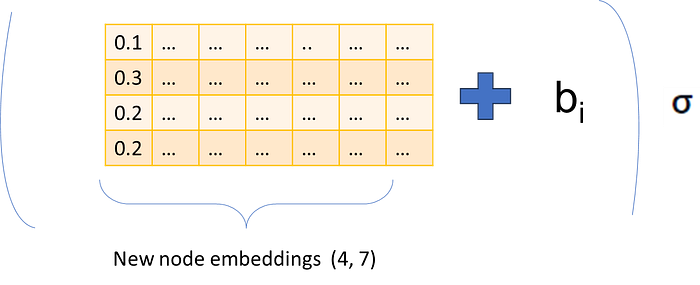
We could say that in this case, the update operation is a sum, however, for other implementations, the update can happen with another learnable function like a linear layer or recurrent neural networks, so another transformation step.
Step 4: Repeat or predict
We could repeat the process, which means stacking several layers of GCN, or we can pool all the node features into a single feature vector to make some prediction on a property of the graph by adding a final fully connected layer.
Similarly, for predictions on specific node or edge properties, we can pool information on neighboring nodes and edges.
An example from PyTorch Geometric
This is an example implementation of GCN extracted from the official page of PyTorch Geometric, where I added an activation function.
Let’s see how the different steps apply here:
import torch
from torch.nn import Linear, Parameter, ReLU
from torch_geometric.nn import MessagePassing
from torch_geometric.utils import add_self_loops, degree

class GCNConv(MessagePassing):
 def __init__(self, in_channels, out_channels):
 super().__init__(aggr='add') # "Add" aggregation (Step 5).
 self.lin = Linear(in_channels, out_channels, bias=False)
 self.bias = Parameter(torch.empty(out_channels))
 self.activation = ReLU()

 self.reset_parameters()

 def reset_parameters(self):
 self.lin.reset_parameters()
 self.bias.data.zero_()

 def forward(self, x, edge_index):
 # x has shape [N, in_channels]
 # edge_index has shape [2, E]

 # Step 1: Add self-loops to the adjacency matrix.
 edge_index, _ = add_self_loops(edge_index, num_nodes=x.size(0))

 # Step 2: Linearly transform node feature matrix.
 x = self.lin(x)

 # Step 3: Compute normalization.
 row, col = edge_index
 deg = degree(col, x.size(0), dtype=x.dtype)
 deg_inv_sqrt = deg.pow(-0.5)
 deg_inv_sqrt[deg_inv_sqrt == float('inf')] = 0
 norm = deg_inv_sqrt[row] * deg_inv_sqrt[col]

 # Step 4-5: Start propagating messages.
 out = self.propagate(edge_index, x=x, norm=norm)

 # Step 6: Apply a final bias vector.
 out += self.bias
 out = self.activation(out)
 return out

 def message(self, x_j, norm):
 # x_j has shape [E, out_channels]

 # Step 4: Normalize node features.
 return norm.view(-1, 1) * x_j
Step 1: Transform
We transform the feature matrix with a linear layer or a learnable weight since we are not using bias
x = self.lin(x)
Step 2: Aggregate
We have to add the self-loop first to the adjacency matrix (in this case represented as a sparse COO format) then we multiply the normalized connectivity matrix by the feature matrix (X). Even though it is in a different format, the resulting operation is the same.
# Step 1: Add self-loops to the adjacency matrix.
edge_index, _ = add_self_loops(edge_index, num_nodes=x.size(0))

# Normalize the connectivity data
row, col = edge_index
deg = degree(col, x.size(0), dtype=x.dtype)
deg_inv_sqrt = deg.pow(-0.5)
deg_inv_sqrt[deg_inv_sqrt == float('inf')] = 0
norm = deg_inv_sqrt[row] * deg_inv_sqrt[col]

# Step 4-5: Start propagating messages.
out = self.propagate(edge_index, x=x, norm=norm) # this calls to the message function

def message(self, x_j, norm):
 # x_j has shape [E, out_channels]
 # Step 4: Normalize node features.
 return norm.view(-1, 1) * x_j
Step 3: Update
We apply the bias and the activation function to update the node embeddings.
# Step 4-5: Start propagating messages.
out = self.propagate(edge_index, x=x, norm=norm) # this calls to the message function
# Step 6: Apply a final bias vector.
out += self.bias
out = self.activation(out)
Conclusion
Just remember that GCNs have 3 steps, and the steps are more or less shared by different GNN architectures like the GAN with small modifications.
- Transformation: Where the node features are transformed by a weight matrix
- Aggregation: Where the different neighboring nodes are summed and normalized.
- Update: Where bias and the activation function are applied to the aggregated features.
Thank you for reading my post, and I hope it has helped you better understand how GNNs work.
Resources
- Understanding Graph Attention Networks: https://www.youtube.com/watch?v=A-yKQamf2Fc&t=113s
- A Gentle Introduction to Graph Neural Networks: https://distill.pub/2021/gnn-intro/
- Creating Message Passing Networks: https://pytorch-geometric.readthedocs.io/en/latest/notes/create_gnn.html
- Graph: Implement a MessagePassing layer in PyTorch Geometric: https://zqfang.github.io/2021-08-07-graph-pyg/
Join thousands of data leaders on the AI newsletter. Join over 80,000 subscribers and keep up to date with the latest developments in AI. From research to projects and ideas. If you are building an AI startup, an AI-related product, or a service, we invite you to consider becoming a sponsor.
Published via Towards AI
Towards AI Academy
We Build Enterprise-Grade AI. We'll Teach You to Master It Too.
15 engineers. 100,000+ students. Towards AI Academy teaches what actually survives production.
Start free — no commitment:
→ 6-Day Agentic AI Engineering Email Guide — one practical lesson per day
→ Agents Architecture Cheatsheet — 3 years of architecture decisions in 6 pages
Our courses:
→ AI Engineering Certification — 90+ lessons from project selection to deployed product. The most comprehensive practical LLM course out there.
→ Agent Engineering Course — Hands on with production agent architectures, memory, routing, and eval frameworks — built from real enterprise engagements.
→ AI for Work — Understand, evaluate, and apply AI for complex work tasks.
Note: Article content contains the views of the contributing authors and not Towards AI.
Related posts
Recent Posts


")


