WORLD OF CLASSIFICATION IN MACHINE LEARNING

Author(s): Data Science meets Cyber Security

Originally published on Towards AI the World’s Leading AI and Technology News and Media Company. If you are building an AI-related product or service, we invite you to consider becoming an AI sponsor. At Towards AI, we help scale AI and technology startups. Let us help you unleash your technology to the masses.

World of Classification in Machine Learning

SUPERVISED MACHINE LEARNING — PART 1

1. CLASSIFICATION:

Classification is the act of categorizing something, as the name implies. Putting it more analytically, classification is the process of categorizing data into classes to gain a better understanding of it. Classification is a type of supervised learning method which can be applied to both structured and unstructured data.

So what exactly we are trying to do is, Use classification to predict the future outcomes of given data points by based on the likelihood and probability of which category they will fall into!

Honestly, the only question now is, How and What can be done to classify data more precisely to be able to understand it better?

Let’s take a simple example of ONLINE DATING!

According to 2022 studies, there are over 8000 dating apps and sites available worldwide, with 323 million users. Isn’t it huge? In the meantime, this application promises 323 million users the right life partner for them based on their common traits, and the users expect a perfect future partner to start a family, have children, live happily, and have fun.

First and foremost, all of these dating apps use an amazing combination of artificial intelligence and machine learning to generate personalized matches, but how does the app know what common traits those matches share? The answer is most likely classification.

If you are one of the 323 million people, you are familiar with the dating app, but for those who aren’t, here is a good example:

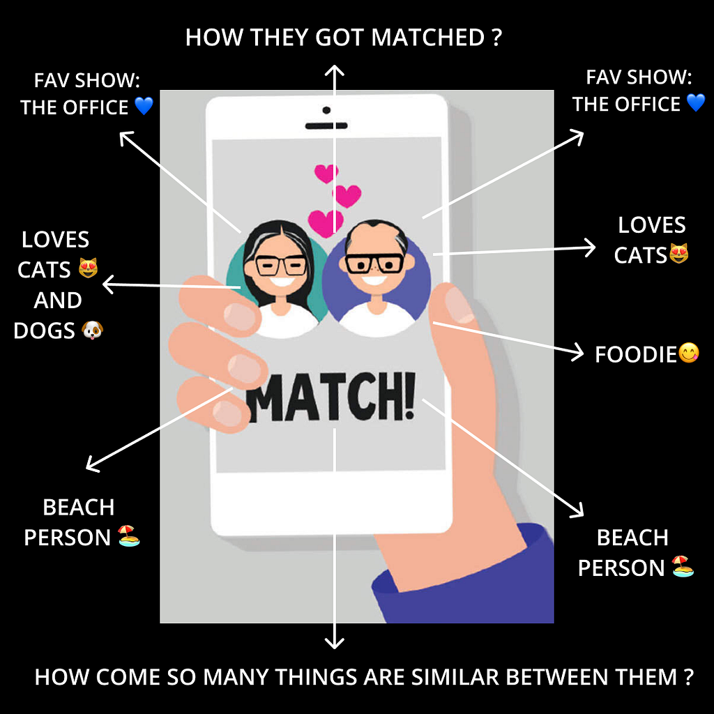
For instance, imagine a User interface with a stack of people, and now you swipe right if you like the person on the screen and left if you don’t. Psychologically, every curious human mind won’t stop by only swiping on 1 person, so when you’re in this process of swiping:

1. Consider you’re swiping right on profiles who have mentioned “THE OFFICE”, as their favorite show
2. Now what the application does is it will classify people from the stack who has “THE OFFICE” as their favorite show (one of many traits)
3. And, in a few seconds, you would be able to see maximum profiles who have mentioned “THE OFFICE” as their favorite show.

So, machine learning is classifying your recommendations based on the traits they believe you prefer, but in reality, it won’t even matter! This is how classification works; it can be based on a variety of characteristics; as we spoke, the above was just a general example to provide context.

TYPES OF CLASSIFICATION TECHNIQUES WHICH ARE USED IN MACHINE LEARNING:

LOGISTIC REGRESSION:

Let’s see some of the problems where Logistic regression can be used to find the solutions.

1. Increasing the reach, followers, likes, and comments on Instagram
2. To predict the future stock price movement.
3. To predict if a patient will get diabetes or not.
4. To classify a mail as spam or non-spam.

LET’S TAKE A LOOK AT THE CASE STUDIES:

CASE STUDY 1:] Suppose based on income levels I want to predict or classify whether a person is going to buy my product or not buy my product.

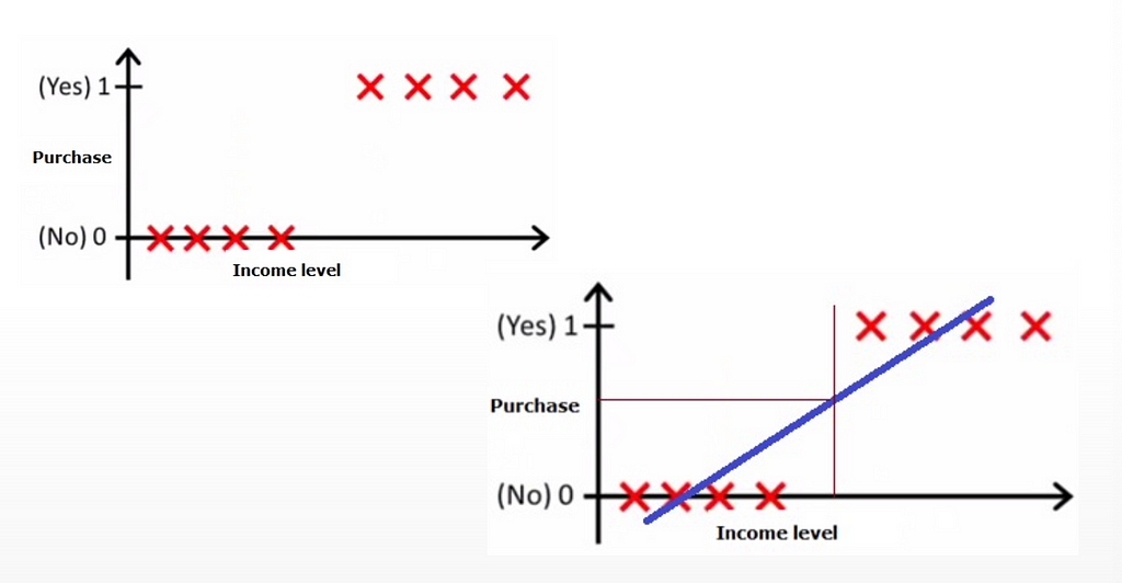
LITTLE DESCRIPTION TO UNDERSTAND THINGS BETTER:

1. The left graph depicts the number of people who would buy the product as 1.
2. The people who will not buy the product because of their income are represented as 0 in the right graph.
3. Now, we can see in the right graph that there is a line drawn on purchase, which we can think of as a threshold value.
4. So the threshold value simply means that people who are inside the line have a low income and cannot afford the product, whereas people who are outside the line have a higher income and can afford the product.

CASE STUDY 2:] We want to plot a graph of the average number of times people have shopped per month and how much money they have spent on each purchase:

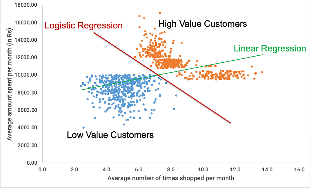
LITTLE DESCRIPTION TO UNDERSTAND THINGS BETTER:

1. So we can see that linear regression is incapable of distinguishing between High Value and Low-Value customers.
2. Linear regression output values are always in the range [-∞, ∞ ], whereas the actual values (i.e., binary classification) in this case are limited to 0 and 1.
3. This is insufficient for such classification tasks; we also require a function that can output values between 0 and 1.
4. This is enabled by a sigmoid or a logistic function, hence the name LOGISTIC REGRESSION.

NAIVE BAYES CLASSIFIER:

Let’s have a look at some of the Classification problems with multiple Classes:

1. Given an article, predict which genre of the newspaper (i.e., Current news, International, Arts, Sports, fashion, etc.) it is supposed to be published in.
2. Given a photo of the car number plate, identifying which country it belongs to.
3. Given an audio clip of the song, identify the genre of the song.
4. Given an email, predicting whether the email is fraud or not.

MATHEMATICALLY SPEAKING:

PROBLEM:

Given certain evidence X, what is the probability that this is from class Yi, i.e, P(Yi|X)

SOLUTION:

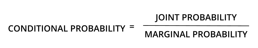
Naive Bayes makes predictions — P(Yi|X) — using Bayes theorem after estimating the joint probability distribution of X and Y, i.e. P(X and Y)

K-NEAREST NEIGHBOR (KNN CLASSIFIER)

To better understand what the KNN algorithm does, consider the following real-world application:

1. KNN is a beautiful algorithm used in recommendation systems.

1. KNN is a beautiful algorithm used in recommendation systems.

3. KNN can search for similarities between two documents and is known as a vector.

This reminds me again of dating apps that use recommendation engines to analyze profiles, user likes, dislikes, and behaviors and provide recommendations to find a perfect match for them.

Take TINDER as an example: Tinder employs a VecTec, a machine learning and artificial intelligence hybrid algorithm that assists users in generating personalized recommendations. Tinder users are classified as Swipes and Swipers, according to Tinder’s chief scientist Steve Liu.

That is, every swipe made by a user is marked on an embedded vector and is assumed to be one of the many traits of the users. (like favorite series, food, educational background, hobbies, activities, vacation destination, and many others)

When the recommendation algorithm detects similarity between the two built-in vectors (two users with similar traits), it will recommend them to each other. (IT’S DESCRIBED AS A PERFECT MATCH!)

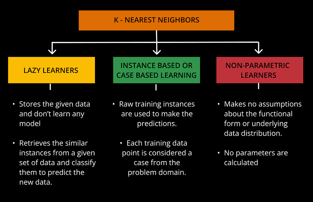
• K-Nearest Neighbors are one of the most basic forms of instance learning

TRAINING METHODS INCLUDE:

• Saving the training examples.

AT PREDICTION TIME:

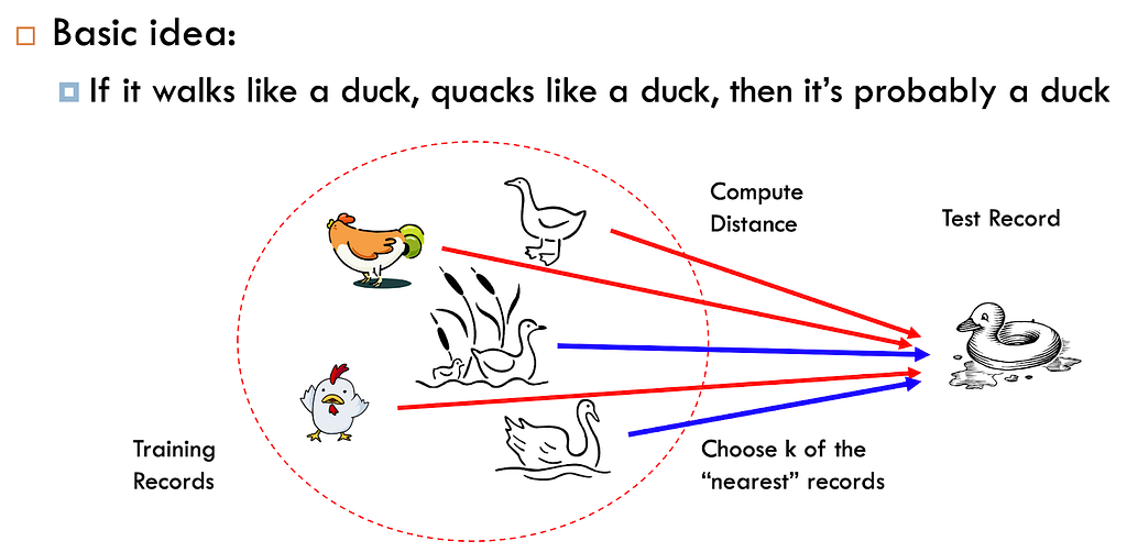
• Find the ‘k’ training examples (x1, y1), and…(xk, YK) that are closest to the test example x. Predict the most frequent class among those yi.

Got this amazing example from the internet where the author explains the KNN algorithm in the most basic way i.e., If it walks like a duck, and quacks like a duck, then it’s probably a duck.

KNN IS FURTHER DIVIDED INTO 3 TYPES:

DECISION TREES:

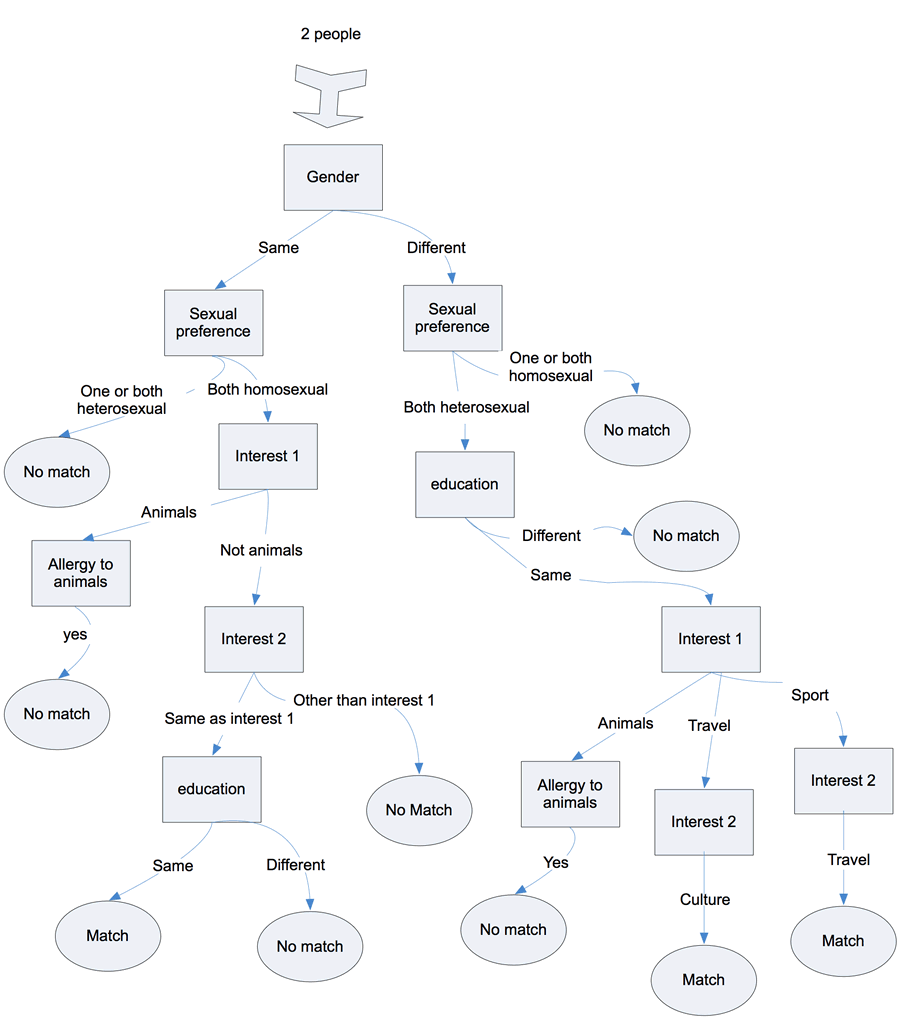
Decision trees are a game-changing algorithm in the world of prediction and classification. It is a tree-like flowchart in which each internal node represents a test on an attribute, each branch represents the test’s outcome, and each leaf node holds a class label.

DECISION TREES TERMINOLOGIES TO UNDERSTAND THINGS BETTER:

ROOT NODE:

→ The decision tree begins at the root node. It represents the entire dataset, which is then split into two or more homogeneous sets.

In our example, the root node is 2 people

LEAF NODE:

→ Leaf nodes are the tree’s final output node, and the tree cannot be further separated after obtaining a leaf node.

In our example, the leaf node ends in a match or no match

SPLITTING:

→ In splitting, we divide the root node into further sub-nodes, i.e., classifying the root node.

In our example, splitting sub-nodes are characteristics like gender, animals, travel, sport, culture, etc.

SUB-TREE:

→ A tree created by splitting another tree

In our example, the sub-tree is Sexual preference, Allergic to animals, or education.

PRUNING:

→ Pruning is the removal of undesirable branches from a tree.

PARENT/ CHILD NODES:

→ The root node of the tree is called the parent node, and other nodes are called the child nodes.

In our example, the 2 people are considered the root node, and the other sub-nodes are considered the child nodes.

SUPPORT VECTOR MACHINES:

The SVM algorithm’s goal is to find the best line or decision boundary for categorizing n-dimensional space so that we can easily place new data points in the correct category in the future. A hyperplane is the best decision boundary.

SVM chooses the exceptional pts, which will help create the higher dimensional space. These extreme cases are referred to as support vectors, and the algorithm is known as the Support Vector Machine.

LET’S TAKE THE SVM PARAMETER — C

1. Controls training error.
2. It is used to prevent overfitting.
3. Let’s play with C.

METHODS TO CALCULATE THE CLASSIFICATION MODEL PERFORMANCE:

CONFUSION MATRIX METHOD:

LET’S UNDERSTAND IT THROUGH AN INTERESTING ANALOGY

Before going deep into how the confusion matrix works, Let’s start with the definition:

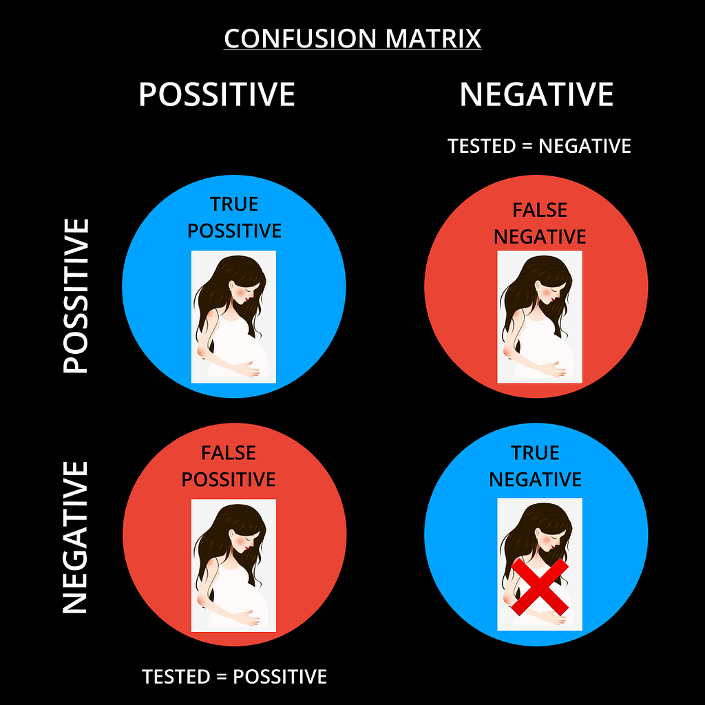
The confusion matrix helps us to determine the performance of the classification models for a given test data. The name is confusing because it makes things easy for us to see when the system is confusing the two classes.

EXAMPLE TO MAKE IT QUICK AND EASY:

ASSUME,

X = The test data of ladies who have come for the checkup.

P = The set of ladies whose test is positive, i.e., they are pregnant.

NP = The set of ladies whose test is negative, i.e., They are not pregnant.

Let x = be the lady who is pregnant from the given set of test data X.

CASE1:] How to calculate how many ladies have POSITIVE results, i.e. P :

P = { x ∈ X: x is pregnant }

CASE2:] How to calculate how many ladies have NEGATIVE results, i.e. NP :

NP = { x ∈ X: x is not pregnant }

POSSIBILITIES OF THE ABOVE CASE STUDIES:

1] A LADY WHO IS PREGNANT AND HER TEST IS ALSO POSITIVE.

Lady ‘A’ is in set ‘X,’ and she tested positive for pregnancy and is pregnant → This is what we call TRUE POSITIVE

2] A LADY WHO IS NOT PREGNANT AND HER TEST IS ALSO NEGATIVE.

Lady ‘A’ is in set ‘X’ and she tested NEGATIVE for pregnancy and is NOT pregnant → This is what we call TRUE NEGATIVE

3] A LADY WHO IS PREGNANT, BUT HER TEST IS NEGATIVE.

Lady ‘A’ is in set ‘X’ and she tested negative for pregnancy, but she is pregnant → This is what we call a FALSE NEGATIVE

4] A LADY WHO IS NOT PREGNANT, BUT SHE TESTS POSITIVE.

Lady ‘A’ is in set ‘X’ and she tested positive for pregnancy, but she is NOT pregnant → This is what we call a FALSE POSITIVE

NOW, THIS IS THE SITUATION WHERE THE CONFUSION MATRIX ENTERS:

A confusion matrix would work and analyze the above situation in the classification algorithm.

The benefit of a confusion matrix is that it helps you to understand your classification model and can predict what exactly the results are and if they are accurate or not, adding to it confusion matrix also helps to find out the errors the model is making

PRECISION AND RECALL METHOD:

Let’s take a simple example to understand this method. Trust me, it’s super easy and exciting.

CASE STUDY 1:] Assume there are two types of malware, which are classified as Spyware and Adware. Now, we’ve created a model that can detect malware in a variety of business software. To do so, we must examine the predictions of our machine learning models.

MODEL 1: TRUE POSITIVE = 80, TRUE NEGATIVE = 30, FALSE POSITIVE = 0, FALSE NEGATIVE = 20

MODEL 2: TRUE POSITIVE = 90, TRUE NEGATIVE = 10, FALSE POSITIVE = 30, FALSE NEGATIVE = 0

As we can see, the false positive rate in model 1 is zero because we don’t want our model to detect the wrong type of malware and cause confusion between the two groups of malware. And as we can see, model 1 has a higher precision value, so let’s start there.

PRECISION = TRUE POSITIVE / TRUE POSITIVE + FALSE POSITIVE

Moving on, in an extreme cyber war, we want to detect malware as soon as possible while keeping their groups apart, and we can see that model 2 has 0 false negatives, which means we can deal with situations where the model does not need to categorize it into two groups of malware, but just detect it so we can put an end to the cyber war as soon as possible. This is also referred to as the RECALL method.

RECALL METHOD = TRUE POSITIVE / TRUE POSITIVE + FALSE NEGATIVE

F -1 SCORE:

Assume you’ve started a paper company, and it’s making less money at first because it’s new. However, you already have a large amount of paper and need a proper place to store that paper as well as an office where you can hire a sales team to increase your sales. Now that we don’t know how many days, weeks, or months the sales will take to complete the sales. So how to predict the deadline?

We need to create a model with a higher F-1 Score which is calculated based on the recall and precision values that can predict that for us.

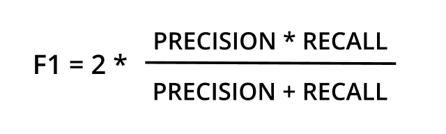
THE HIGHER THE F-1 SCORE, THE BETTER THE MODEL

FOLLOW US FOR THE SAME FUN TO LEARN DATA SCIENCE BLOGS AND ARTICLES:💙

LINKEDIN: https://www.linkedin.com/company/dsmcs/

INSTAGRAM: https://www.instagram.com/datasciencemeetscybersecurity/?hl=en

GITHUB: https://github.com/Vidhi1290

TWITTER: https://twitter.com/VidhiWaghela

MEDIUM: https://medium.com/@datasciencemeetscybersecurity-

WEBSITE: https://www.datasciencemeetscybersecurity.com/

-Team Data Science meets Cyber Security ❤️

---

WORLD OF CLASSIFICATION IN MACHINE LEARNING was originally published in Towards AI on Medium, where people are continuing the conversation by highlighting and responding to this story.

Join thousands of data leaders on the AI newsletter. It’s free, we don’t spam, and we never share your email address. Keep up to date with the latest work in AI. From research to projects and ideas. If you are building an AI startup, an AI-related product, or a service, we invite you to consider becoming a sponsor.

Published via Towards AI