Why Most Introductory Examples of Bayesian Statistics Misrepresent It

Author(s): Ruiz Rivera

Originally published on Towards AI the World’s Leading AI and Technology News and Media Company. If you are building an AI-related product or service, we invite you to consider becoming an AI sponsor. At Towards AI, we help scale AI and technology startups. Let us help you unleash your technology to the masses.

If you’ve ever come across material that introduces Bayesian Inference, you’ll find that it usually involves an example of how misleading some medical testing devices can be in detecting diseases. Other variations of this example include using a breathalyzer to detect the amount of alcohol in the bloodstream or if we want to get creative, some fictional device that can distinguish an ordinary person from a werewolf. You get the idea. These examples involve providing the reader with a few critical variables/constants that are necessary for plugging into Bayes’ Theorem, such as:

• The prevalence of the disease in the population, which we’ll define as our prior, or the probability of the hypothesis P(H):
  → P(H)=0.001 (i.e., there is 1 person carrying the disease out of every 1,000 people)
• The True Positive Rate (TPR) of the medical test, which is the probability that the device will RETURN POSITIVE, indicating that it thinks you have the disease, given (represented by “∣” ) the fact that you are ACTUALLY INFECTED with it:
  → P(E ∣ H) = 0.95 (i.e., the device will correctly identify 95 out of 100 people who are carrying the disease)
• The False Positive Rate (FPR) of the medical test, which is the probability that the device will RETURN POSITIVE, indicating that you have the disease, given the fact that you are ACTUALLY NOT INFECTED:
  → P(E ∣ H−) = 0.01 (i.e., the device will incorrectly label 1 person as infected out of 100 people who don’t carry the disease)

Another key component in Bayes’ Theorem that isn’t explicitly defined, but is equally necessary to be aware of, is the Probability of the Evidence, also known as the Marginal or Average Likelihood. The average likelihood uses the Law of Total Probability, which states that the outcome of ALL events must equal 1, thus quantifying the probability of the evidence being true. Its job is to standardize the posterior in order to get a probability of a certain event coming true. For example, if we’re expecting a binomial distribution from the posterior, such as the probability of being infected vs. not infected or the probability of a coin landing on heads vs. tails, we can generate the average likelihood by adding both probabilities together:

• ***Note that Pr(H-), which is the probability of you NOT carrying the disease, was the only variable we didn’t provide. However, we can easily calculate it by subtracting it from 1: Pr(H-) = 1 — Pr(H)

After providing the necessary constants, the question we’re often left with to illustrate the use of Bayes’ Theorem is the following:

What is the probability that you TEST POSITIVE for carrying the disease given the fact that you are ACTUALLY INFECTED?

This is a trick question because most people will answer it with the TPR of the medical device (95%) without considering the disease’s prevalence in the wider population. In the case of TPR, the information it contains is kind of the opposite of the question we’re asking because TPR assumes that you are already infected, so it simply provides you with the probability that the medical test will identify it. So with our “trick question,” what we’re really asking is whether or not you are actually infected with the disease AFTER testing positive for it. At this point, whether or not you are actually carrying the disease is still unknown and is ultimately the question we’re trying to answer.

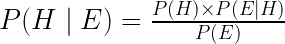
And it’s here where the mythical Bayes’ Theorem is introduced as the mathematical solution which uses the evidence available to us (represented as P(E)) to update our prior beliefs (represented as P(H)), resulting in new and updated posterior beliefs. Thus, we can express the idea of Bayes’ Theorem using the mathematical equation:

To those still a bit shaky with Bayesian Statistics, let’s delve a little deeper into the philosophy behind this alternative universe. Bayesian Statistics is what many consider to be another philosophy towards statistics and probability, which allows the practitioner to integrate their lived experience or prior knowledge towards a question they are trying to answer using data. Generally speaking, the Bayesian approach to probability posits that we can increase our understanding of a topic of interest by updating our prior knowledge based on the evidence (i.e., the data) we come across. So the more data and information we have about our particular topic, the stronger we can cement our beliefs based on the observations we’ve experienced. In contrast, if we have a solid prior knowledge base on a topic we’re studying, it would take substantially more data/evidence to change our long-standing beliefs. In some sense, the Bayesian method of updating information closely mimics the process of scientific inquiry in using observations to form and/or update our body of knowledge.

And, of course, it would be remiss to at least mention how the Bayesian view of probability juxtaposes the Frequentist view of probability which is often the default perspective of statistics taught in schools. From the Frequentist perspective on probability, there is an objective ground truth to a phenomenon we’re interested in, which we get a clearer picture of as we increase our sample size. Frequentists view probability as a property of a repeatable event, NOT as a subjective belief or a prior hypothesis. So, for example, if we flip a coin 100 times and it lands on heads 50 times, then a Frequentist would interpret that the coin has an objective, associated property of landing on heads 50% of the time. In contrast to the Bayesian approach, Frequentists do not assign probabilities to pre-existing hypotheses or models, so in some sense, they approach every problem as a blank slate. In their view, probability statements about an event or a hypothesis are either true or false based on the observed data.

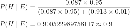
Going back to our medical testing case study, the constants provided at the beginning represent our priors, which we’ll use to update our beliefs based on our medical test results. As we’ll often find out at the end of the demonstration, if we input the constants provided, we’ll discover that the chances of truly carrying the disease after our medical test indicated we were infected is actually very low:

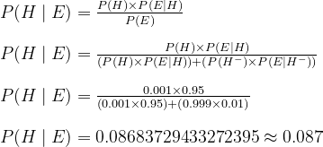
While it’s often surprising that the chances we could be infected with this disease after testing positive for it is only about 9%, the workaround for that is repeated testing. If we take that same medical test a second time and it INDICATES that we’re carrying the disease, then there’s about a 90% chance that we are ACTUALLY INFECTED. To do this, all we have to do is run the same calculation but instead, update our new prior with the posterior we just solved for P(H) = 0.087:

Now that we’ve gone through a brief overview of how Bayes’ Theorem works let’s now try to parse out why this common example misrepresents the Bayesian interpretation of probability. One of the biggest reasons why I disagree with the common technique of highlighting Bayes’ Theorem to introduce Bayesian Statistics is because we used fixed constants (i.e., P(H)=0.0001 or TPR=0.95, etc.) in our example to generate our posteriors so there’s nothing uniquely “Bayesian” about it (McElreath, 2020). Simply put, the thing that distinguishes Bayesian Inference from other interpretations of probability is by its broad use of probability to generate posteriors, NOT by its use of Bayes Theorem (McElreath, 2020). Bayesian Inference allows us to consider a range of possible outcomes rather than just a single-point estimate, which is useful in situations where there is uncertainty or ambiguity about the true state of the world. To clarify, the term “point estimates “ is simply a Bayesian term for the “fixed constants” we defined at the beginning of our example, such as the TPR of our medical tests. Point estimates often come up in Bayesian literature to describe the idea that taking a single number to represent an entire distribution of outcomes can be harmful because we would lose all of the information and the nuance associated with said outcomes. Regardless of how we love to simplify things to easily fit our mental models, the worlds that we are studying are inherently messy and ambiguous. By considering the entire range of outcomes or probabilities, Bayesian Inference then allows us to make more nuanced and accurate predictions.

So with all that said, how can we improve the prior example to illustrate how Bayesian Inference works in the real world? Rather than make assumptions about the probabilities of the prior (0.001) since it can be difficult to get accurate estimates of the disease’s prevalence in a population, instead, we can consider a subset of possible values. And because we’re skeptical about the stated prevalence of the virus, let’s generate our own estimates using a few Python libraries, such as NumPy or Pandas. In this case, we’ll use the code to simulate the range of possible outcomes between where the disease has a low prevalence rate that infects 1 in every 10,000 people (0.0001), and a high prevalence rate that infects 1 in every 10 people (0.1). Each value we generate will serve as a prior from which we’ll map an associated posterior value.

import pandas as pd
import numpy as np
import matplotlib.pyplot as plt
 
# Constants
prior_dist = np.arange(0.0001, 0.1, 0.0001) 
likelihood = 95/100
false_pos = 1/100

Once we have our list of possible values representing the prevalence of the disease in the population, we can generate the probability that you’ve contracted the disease after initially testing positive for it. For example, with the first value in our distribution, we’re asking ourselves the question: Assuming that the disease infects 1 out of 10,000 people (0.0001), what is the probability that we’ve contracted it after testing positive from our medical device? In this example, we’ll find that there’s less than 1% chance we’ve actually contracted the disease (0.9412%) due to the low prevalence of the disease.

# Calculating the posterior distribution
posterior_dist = []
 
for point_est in prior_dist:
  posterior_est = (point_est * likelihood) / ((point_est * likelihood) + ((1-point_est) * false_pos))
  posterior_dist.append(posterior_est)
 
val_dicts = {"priors": prior_dist, "posteriors": posterior_dist}
med_df = pd.DataFrame(val_dicts) # For ease of querying

From then on, we’ll generate the probabilities of contracting the disease after testing positive for it when it’s prevalent in every 2 people out of 10,000, then 3, then 4, and so on until we reach a prior that assumes 1,000 in every 10,000 (in other words, 1 in 10) is infected. Finally, after we’ve generated a posterior distribution, we can graph the relationship between our priors and posteriors and compare where our original point estimate ( p = 0.001) fell within this curve.

fig = plt.figure(figsize=(10, 6), dpi=80)
plt.plot(med_df["priors"], med_df["posteriors"])
plt.scatter(med_df[med_df["priors"] == 0.001]["priors"], med_df[med_df["priors"] == 0.001]["posteriors"], color="red")
plt.ylabel("Posterior Probability $p(disease+ \mid test+)$")
plt.xlabel("Prior Probability $p(disease+)$")
plt.title(f"The probability distribution of catching the disease given that device is  {(100 * likelihood):.0f}% in detecting it")

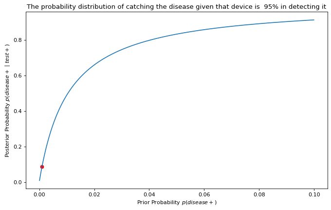
One observation we can make from the graph is that the chance of you contracting the disease after testing positive for it increases exponentially as the disease’s prevalence rate in the population also increases. Of course, this assumes that our medical device is indeed 95% accurate in positively diagnosing a patient who’s already infected. If we were skeptical about this figure, we could also generate a list of possible values for the effectiveness of our medical device, something we can cover in later blog posts.

In taking a probabilistic approach by considering a range of different priors, rather than relying on a single point estimate which is the case for many introductory examples of Bayesian Inference, we remain more faithful to the Bayesian view of probability. That said, educators must not overlook taking a probabilistic approach when introducing Bayesian Statistics. Without it, newer practitioners will naturally form strong priors that Bayes’ Theorem is what defines the entire field of Bayesian Statistical Inference!

References

McElreath, R. (2020). Statistical Rethinking: A Bayesian Course with examples in R and Stan. Routledge. http://xcelab.net/rmpubs/sr2/statisticalrethinking2_chapters1and2.pdf

---

Why Most Introductory Examples of Bayesian Statistics Misrepresent It was originally published in Towards AI on Medium, where people are continuing the conversation by highlighting and responding to this story.

Join thousands of data leaders on the AI newsletter. It’s free, we don’t spam, and we never share your email address. Keep up to date with the latest work in AI. From research to projects and ideas. If you are building an AI startup, an AI-related product, or a service, we invite you to consider becoming a sponsor.

Published via Towards AI