What is the connection between a World Model, Schrödinger’s Cat, and Neural Network?

Author(s): Alexander Kovalenko

Originally published on Towards AI.

What Is the Connection Between a World Model, Schrödinger’s Cat, and Neural Networks?

Using Physics-Informed Neural Network (PINN) to solve famous Schrödinger Equation

For centuries, curious minds have been trying to crack the structure of the world around us. Most would agree that any branch of science follows the same goal — trying to map a function to the observations. This function, which somehow explains the world model by an approximation, can be either continuous or discrete and is meant to find a correspondence between the input and output sets.

The search for a function that describes the world model can be tricky without any prior knowledge. However, we know that the world around us is complex and dynamic. Complex models can be represented by simple rules, so there might be a walkaround. 😅 Nevertheless, as things tend to evolve in time and space, the dynamic aspect of the ever-changing world can’t be simply ignored.

“Something can only ever be explained by taking something else for granted”

Richard Feynmann

Dynamics can be described through a derivative that measures the sensitivity of the function output with respect to changes in the input. At the same time, the relation between the function and its derivative is defined in a form of a differential equation. Therefore, it’s a no-brainer that many phenomena in physics, engineering, economics, biology, psychology, and whatnot can be successfully modeled by using differential equations of any type. Differential equations can be used to calculate the movement or flow of electricity or heat, the motion of an object, or even to check the growth of diseases. Needless to say, the whole backpropagation algorithm can be seen as a differential equation, where the partial derivatives of the error are calculated with respect to weights, using the chain rule.

On the one hand, we have an unknown function; on the other hand, its derivative represents the rate of change. The differential equation defines the relationship between the two.

Even though many of you probably know Erwin Schrödinger by his thought experiment often called “Schrödinger’s Cat”, he is foremost known to be one of the godfathers in the field of quantum theory. Schrödinger postulated the equation (which is now called the Schrödinger equation) that governs the wave function of a quantum-mechanical system or describes where the quantum particle is.

One can even set up quite ridiculous cases. A cat is penned up in a steel chamber, along with the following device (which must be secured against direct interference by the cat): in a Geiger counter, there is a tiny bit of radioactive substance, so small, that perhaps in the course of the hour one of the atoms decays, but also, with equal probability, perhaps none; if it happens, the counter tube discharges and through a relay releases a hammer that shatters a small flask of hydrocyanic acid. If one has left this entire system to itself for an hour, one would say that the cat still lives if meanwhile, no atom has decayed. The first atomic decay would have poisoned it. The psi-function of the entire system would express this by having in it the living and dead cat (pardon the expression) mixed or smeared out in equal parts.

Schrödinger, E. Die gegenwärtige Situation in der Quantenmechanik. Naturwissenschaften 23, 807–812 (1935).

“Schrödinger equation” is one of the fundamental landmarks in understanding quantum physics and building a clearer picture of the world model. And guess what? This equation is a linear partial differential equation as shown below:

Where Ψ is an unknown wave function we want to find. Before we begin, I have to tell you that there is an uncountable number of particular cases of the Schrödinger equation though many of them are prohibitively complex, and thus they can’t be solved analytically for most atoms. Therefore, let’s now concentrate on one of the simplest cases, which is “The Schrödinger equation’s” solution for “particle-in-a-box”, which is a nice demonstration of the differences between classical and quantum systems.

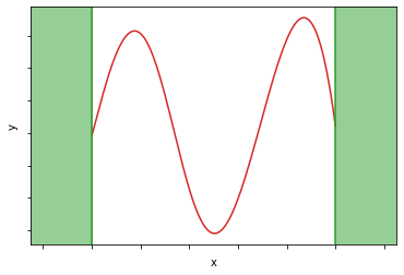
Imagine, our particle is trapped between two infinite potential barriers (this case is sometimes called an infinite potential well). The particle is free to move in between the walls, though. Since this is a very restricted case, in fact, a hypothetical toy example, there are ways to simplify our initial expression, resulting in a time-independent Schrödinger equation for a single particle in the box:

How do we do that? See the amazing video below explaining how to derive a particular case for a particle-in-a-box and solve it analytically:

Nevertheless, we ended up with a second-order differential equation. The Ψ function describes the behavior of the particle. Position, momentum, and energy may be derived from the Ψ. If you’ve already watched the video, you already know how to solve it. However, if you haven’t, it might seem that the equation above does not look so complicated. So what is the problem?!

If we take a closer look, then all we know is that the Ψ(0) = 0, Ψ(a) = 0, and the second derivative of Ψ plus Ψ itself is also zero! However, we know that Ψ is not zero in the interval (0, a).

ಠ益ಠ

Ok, let’s pull all the knowledge we have, except the equation itself, together:

• Ψ is a function;
• Ψ(0) = 0
• Ψ(a) = 0

Since Ψ is a function, and we are data scientists, we can leverage the universal approximation theorem, which roughly states the following:

Once the number of neurons is sufficient, the feedforward neural network with a non-polynomial activation function can approximate any well-behaved function to any accuracy.

This theorem is valid for both multi- and single-hidden layer neural networks, and basically for any of the modern activation functions (ReLU, GeLU, Sigmoid, Tanh, etc.). Seems like exactly what we need!

No… Wait… What about the data?!

Well, we have none. However, there is a way out, called Physics Informed Neural Networks, or PINNs. PINNs attracted particular attention recently, mainly due to their ability to model and forecast the dynamics of multiphysics and multiscale real-world systems. Another interesting property of PINNs is that if we are fitting data that should obey some physical law, and we are aware of this law, we can simply add this dependence to the loss function, which makes our machine learning model respect the physical law, i.e. to be physics informed.

In general, regarding PINNs, we can define three ways we could efficiently train the model:

• lots of data and no physics (what we are all familiar with)
• little data and some physics
• no data and all the physics we have

NB: For the sake of simplicity, we are going to omit all the constants in the equation. We’ll assume that k=1, and our quantum well is from 0 to a=10.

Our case is exactly the third one. We have the physical law to follow, but no data. Let’s define the boundary conditions simply as the function that returns zero:

And since the equation above has no residuals, i.e. all the Ψ containing terms are on the left part, we can define a function for our Schrödinger equation. Simply, it is going to be something that tends to be zero.

Then, as discussed above, a multilayer perception with non-polynomial nonlinearity should be a good option to approximate our wave function Ψ. Here we used Gaussian Error Linear Unit nonlinearity as it was found empirically to work slightly better than Sigmoid and Tanh, while ReLU showed the worst performance.

Consequently, we have to make our model respect Schrödinger’s equation, meaning to be physics informed. This can be achieved by defining the loss function that includes the discrepancy of the whole differential equation and the discrepancy at boundaries:

Note that we can calculate the gradients (or simply the derivative of Ψ function psi_x) by using torch.autograd.grad(), an automatic differentiation function that computes and returns the sum of gradients of outputs with respect to the inputs. To compute the second derivative psi_xx, simply apply grad() function twice.

Therefore, we can pass boundaries at the walls of the box and data points within the box to calculate the overall loss and then backpropagate the error to update the weights.

After a few thousand iterations, we can take a look at the result. As shown below, the output of our function resembles the solution for the particle-in-a-box case. Since we know that the solution for the Schrödinger equation is in fact a family of solutions, the output may vary upon stochastic initialization of weights and training parameters. The complete code can be found here.

Of course, there are many more sophisticated implementations showing how to solve the Schrödinger equation using deep neural networks[1, 2, 3]. On the other hand, this blog post demonstrates a simple and understandable introduction to physics-informed machine learning and gives an idea of when and why we’d like to “inform” our model. The reason I chose Schrödinger’s equation is simple — since the equation itself and boundary conditions are quite restrictive and non very informative (as you remember, zeros were everywhere). The gradient descent algorithm, was able to find a nonzero solution, even though it was not penalized.

Finally, we can answer the question stated in the blog post title: “What is the connection between a World Model, Schrödinger’s Cat, and Neural Network?”. As we know, many dynamic processes describing the world model can be modeled using differential equations. On the other hand, even very complicated differential equations can be solved with physics-informed neural networks.

---

What is the connection between a World Model, Schrödinger’s Cat, and Neural Network? was originally published in Towards AI on Medium, where people are continuing the conversation by highlighting and responding to this story.

Join thousands of data leaders on the AI newsletter. Join over 80,000 subscribers and keep up to date with the latest developments in AI. From research to projects and ideas. If you are building an AI startup, an AI-related product, or a service, we invite you to consider becoming a sponsor.

Published via Towards AI