UNet++ Clearly Explained — A Better Image Segmentation Architecture

Author(s): Leo Wang

Originally published on Towards AI the World’s Leading AI and Technology News and Media Company. If you are building an AI-related product or service, we invite you to consider becoming an AI sponsor. At Towards AI, we help scale AI and technology startups. Let us help you unleash your technology to the masses.

UNet++ Clearly Explained — A Better Image Segmentation Architecture

Table of Contents

∘ ⭐️ U-Net Recap
∘ ⭐️ UNet++ Innovations
∘ ⭐️ Loss function
∘ ⭐️ Performance
· Citations

In this article, we are going to introduce you to UNet++, essentially an upgraded version of U-Net. This article is designed to help you understand it intuitively and thoroughly with minimum time possible. It is recommended that you at least have a very rough idea of what U-Net is, but we are going to do a recap anyways!

⭐️ U-Net Recap

Introduced in 2015, U-Net aimed to conduct image segmentation tasks specifically in the field of medical imaging. Its name is derived from its “U-Shaped” architecture.

The architecture consists of a contracting path (aka. downsampling path, encoder), where the width and heights of the feature maps are shrunk while the channel expands by a factor of 2 until it reaches 1024 (typically the maximum recommended level for CNNs), a bottleneck as a “turning point”, and an expanding path (aka. upsampling path, decoder), where widths and heights of the feature maps are expanded to the mask’s dimension.

⭐️ UNet++ Innovations

“Upgraded” from U-Net, UNet++ essentially added dense convolutional blocks (Fig 1 in blue and Fig. 3) and a deep supervision design (Fig. 2 in red) that nests on the top level of the network. The newly proposed model looks like this:

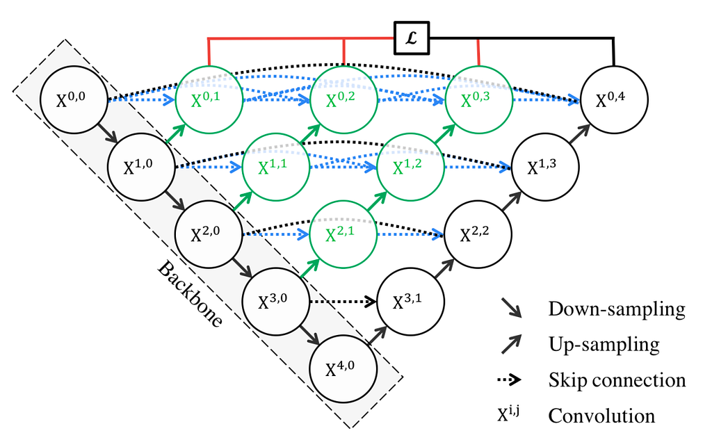
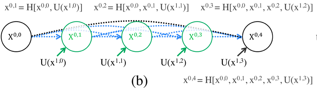
The first design change is added dense convolutional block, Fig. 2 intuitively and concisely shows how it works.

In U-Net, the feature maps generated from the encoder are automatically passed to the decoder at the same level (shown in BLACK in Fig. 3). However, in UNet++ that is changed (as shown in Fig 3 in BLUE and GREEN). To understand it, here’s the explanation:

• In the formula shown at the top of Fig 3, H is DenseNet’s composite function that combines Batch Normalization, ReLU activation, and a 3×3 convolution.
• The elements inside [] are concatenated together as inputs to the H composite function.
• U is U-Net’s composite function; by default, when you use U-Net’s own backbone, you should expect two 3×3 convolutions with ReLU activations (shown in Fig. 1 as how each level is structured).
• It should be noted that the introduced dense blocks in the middle take into not only the information from the previous “nodes,” in the same level but also the “nodes” in the level below it (shown in Fig. 2). This is a really densely connected network!

Therefore, the newly introduced dense connections would help reduce the “semantic gap between the feature maps of the encoder and decoder”(Fig. 1), so the model could have an easier learning task because those feature maps would be more “semantically similar.”

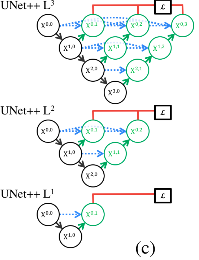
The second change in UNet++ is an added deep supervision design (Fig. 4 in red).

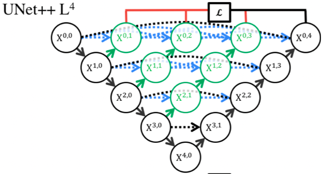
Deep Supervision is not as hard as it seems. Essentially, it helps the model to operate in two modes:
1) Accurate mode (the outputs from all branches in level 0 are averaged to produce the final result)
2) Fast mode (not all branches are selected for outputs)

Figure 5 shows how different choices in FAST MODE result in different models

⭐️ Loss function

In the paper, the author proposed a combined loss function of Binary Cross Entropy and Dice loss, as shown in Formula 1.

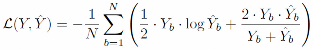
The author used 0.5 weights for BCE loss and 1.0 weights for Dice loss. Note: Dice coefficient is equivalent to F1 score. During implementation, it is suggested to use 1 minus the dice coefficient when using the dice coefficient as a loss. Therefore, this practice shown in the paper maybe is subject to improvement.

Moreover, Dice loss is often hard to converge as its non-convex nature. Therefore, one recent solution is provided by wrapping it in a log and cosh function to “smooth out the curve” (https://arxiv.org/pdf/2006.14822.pdf)

Also, combining BCE loss with Dice loss often leads to better results.

⭐️ Performance

The author trained the model on four different datasets, and all yielded better performances than U-Net and Wide U-Net models. Table 1 shows the result. DS means deep supervision. The result is shown in the IoU score (area of overlap/area of the union), which illustrates how accurate the model is.

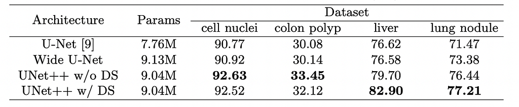
The result demonstrates that UNet++ indeed improved compared to its predecessor U-Net.

Next, we are going to show you how UNet 3+ works. It’s an upgraded version of UNet++!

UNet 3+ Fully Explained — Next UNet Generation

Thank you! ❤️

Citations

[1] Z. Zhou, M. Siddiquee, N. Tajbakhsh, and J. Liang, UNet++: A Nested U-Net Architecture for Medical Image Segmentation (2015), 2015 Computer Vision and Pattern Recognition
[2]: O. Ronneberger, P. Fischer, and T. Brox, U-Net: Convolutional Networks for Biomedical Image Segmentation (2015), 2015 Computer Vision and Pattern Recognition

UNet++ Clearly Explained — A Better Image Segmentation Architecture was originally published in Towards AI on Medium, where people are continuing the conversation by highlighting and responding to this story.

Join thousands of data leaders on the AI newsletter. It’s free, we don’t spam, and we never share your email address. Keep up to date with the latest work in AI. From research to projects and ideas. If you are building an AI startup, an AI-related product, or a service, we invite you to consider becoming a sponsor.

Published via Towards AI