Understanding every bit of Dummy Variables — Must for AI and ML engineers

Author(s): Supriya Ghosh

Originally published on Towards AI the World’s Leading AI and Technology News and Media Company. If you are building an AI-related product or service, we invite you to consider becoming an AI sponsor. At Towards AI, we help scale AI and technology startups. Let us help you unleash your technology to the masses.

Understanding every bit of Dummy Variables — Must for AI and ML Engineers

Introduction

Dummy variables are widely used in Data Science and Machine Learning due to the qualitative nature of dependent and independent variables. Qualitative includes categorical variables which mean variables can be classified into different categories. In this write-up, I will discuss in detail all concepts of dummy variables.

Topic Map

1. Dummy Variables definition and introduction

2. A linear regression case with 1 qualitative variable (consisting single dummy variable) and 1 quantitative variable, with no interaction variable considered.

3. Linear regression case with 1 qualitative variable (consisting double-dummy variables) and 1 quantitative variable.

4. Linear regression case with 1 dummy variable and 1 quantitative variable with interaction variable considered.

5. One-hot encoding concept and Dummy variable trap.

What are dummy variables?

Dummy variables are qualitative variables or discrete variables that represent categorical data and can take the values as 0 or 1 to indicate the absence or presence of a specified attribute respectively.

Dummy variables are also known as indicator variables, design variables, and binary basis variables.

They are used frequently in the time-series analysis along with seasonal component analysis, linear regression models, and many other applications where qualitative data is predominant.

In general, the explanatory variables or the independent variables in any regression analysis are assumed to be quantitative in nature. For example, variables like temperature, distance, age, etc. are quantitative in the sense that they are measured on a well-defined scale.

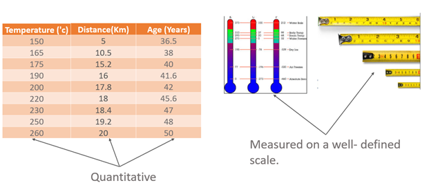
But in many applications, the variables cannot be measured on a defined scale, and they are qualitative in nature.

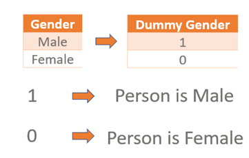
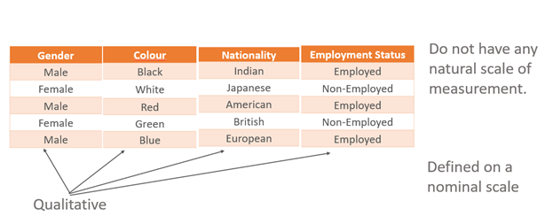
For example, the variables like sex (male or female), color (black, white), nationality, and employment status (employed, unemployed) are defined on a nominal scale. Such variables do not have any natural scale of measurement. Such variables usually indicate the presence or absence of a “quality” or an attribute like employed or unemployed, graduate, or non-graduate, smokers, or non-smokers, yes or no, acceptance or rejection, so they are defined on a nominal scale. Such variables can be quantified by artificially constructing the variables that take the values, e.g., 1 and 0 where “1” indicates usually the presence of an attribute and “0” usually indicates the absence of an attribute. For example, “1” can indicate that the person is male, and “0” can indicate that the person is female.

Similarly, “1” may indicate that the person is employed and then “0” may indicate that the person is unemployed. Such variables classify the data into mutually exclusive categories. These variables are called indicator variables or dummy variables.

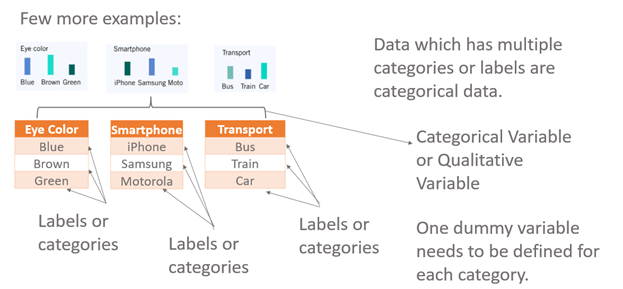
The point to note here is: — Where a qualitative variable has two or more two categories, it can be represented by a set of dummy variables, with one variable for each category.

Numeric variables can also be dummy coded to explore nonlinear effects. But there are certain disadvantages to it like :

Treating a quantitative variable as a qualitative variable increases the complexity of the model. The degrees of freedom for error is also reduced. This can affect the inferences if the data set is small. In large data sets, however, such an effect may be small.

Example of dummy variable –

Let us consider an example to elaborate concept in detail through a case of Linear Regression.

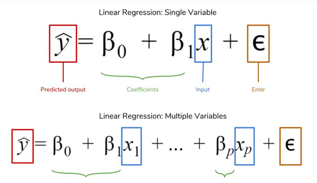
Linear Regression equation

Use Case 1

We have 2 explanatory variables/independent variables and 1 response /dependent variable.

Explanatory variables — Gender and Age.

Gender is a qualitative independent variable with 2 categories (Male and Female)

And a dummy variable corresponding to Gender is depicted as DGender

Here, 1 dummy variable for 2 categories (Male and Female) for the qualitative independent variable is considered.

Age is quantitative (numeric) independent variable depicted as X.

Response variable — Salary

It is a quantitative (numeric) response or dependent variable and is depicted as Y.

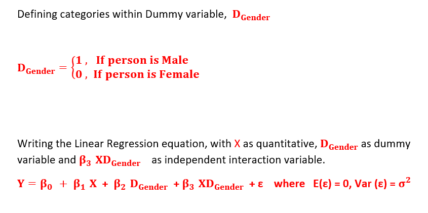
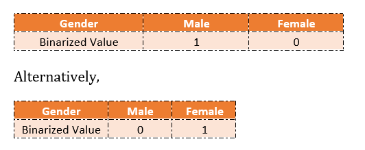
Defining categories within the Dummy variable, DGender

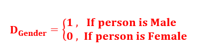
The below table represents the depiction.

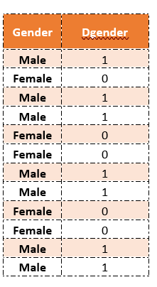
This takes values as 0 and 1 to identify the mutually exclusive class.

It is not necessary to choose only 1 and 0 to denote the category. In fact, any distinct value of DGender will serve the purpose. The choices of 1 and 0 are preferred as they make the calculations simpler and help in the easy interpretation of the values. But the results derived are the same whether you consider values as 1 and 0 or -1 or 1 or 1 and 2 etc.

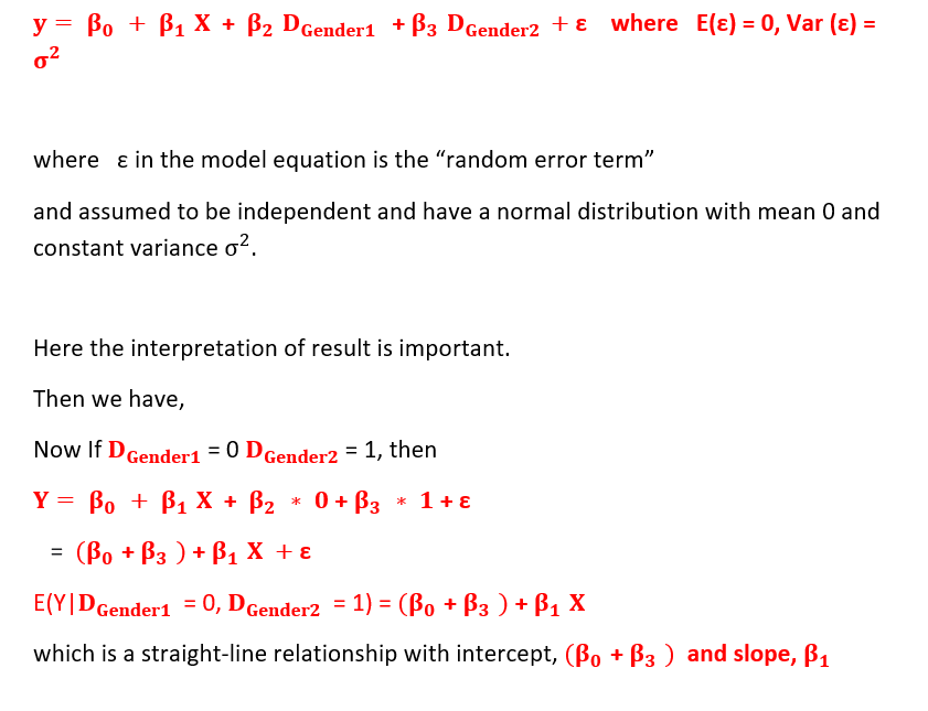
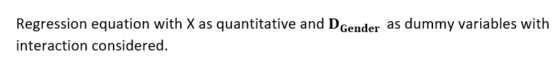
Writing the Linear Regression equation, with X as quantitative and DGender as a dummy variable.

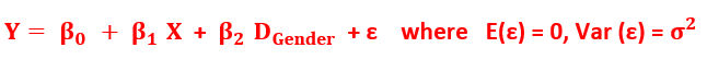
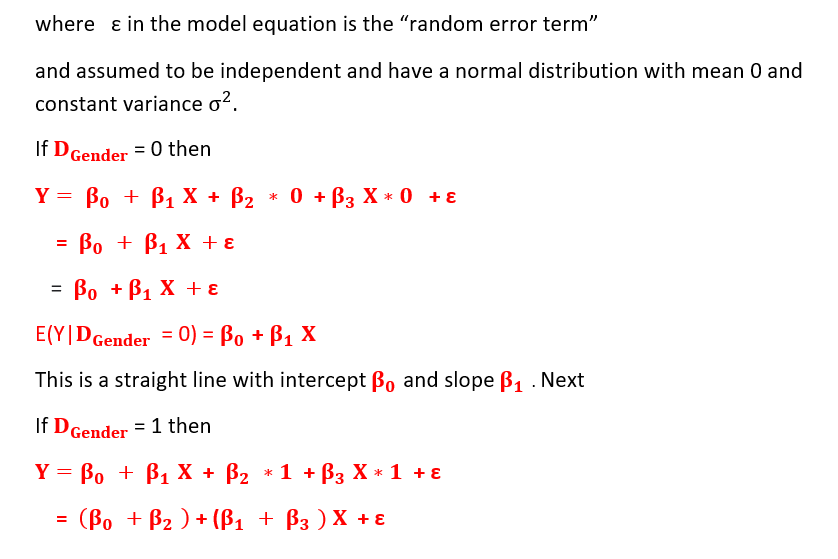
where ε in the model equation is the “random error term”

and assumed to be independent and have a normal distribution with mean 0 and constant variance.

Here the interpretation of the result is important.

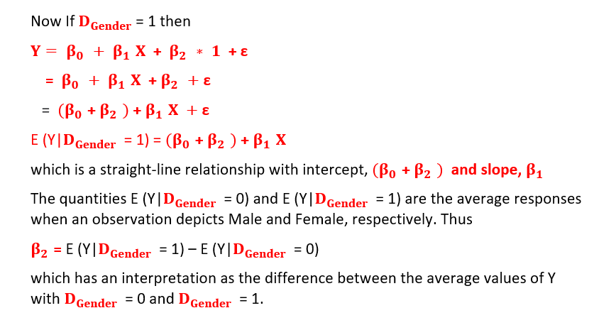
We proceed as follows:

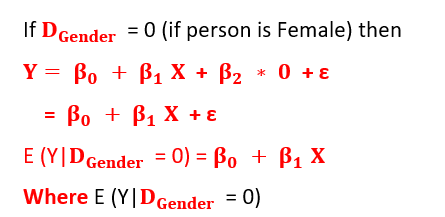
represents a change in mean response in E(y) with per unit change (here unit change means a change from 0 to 1 or 1 to 0 since values are binary) in the associated dummy predictor variable when all the other predictors are held constant.

So this is a straight-line relationship with intercept, bo, and slope, b1.

Graphically, it looks like the below figure. It describes two parallel regression lines with the same variances.

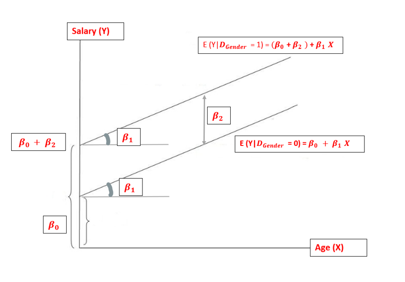
Regression equation with X as quantitative and DGender as dummy variable

Two parallel lines suggest the absence of any significant interaction amongst independent variables i.e., the effect of the dummy explanatory variable, Gender on the response variable, i.e., salary is the same at different values of the other explanatory variable i.e. age.

This is a very important conclusion in itself as it affects the model created significantly and if interaction effects exist, it makes the model more complex in terms of results interpretation.

Interaction effects in general indicate that a third variable influences the relationship between an independent and dependent variable.

Point to note: Generally, n-1, dummy variables are created for n categories i.e. in our example of Gender, where Gender has 2 categories (Male and Female), only one dummy variable DGender is created.

Why n — 1 dummy variables are created for n categories, not n is an interesting topic that I will cover in a subsequent section.

Let’s start off with our 2nd case :

Let me consider the same example as above but now I consider 2 dummy variables for 2 categories (Male and Female) for the qualitative independent variable. All other things remain the same.

Also, no interaction is considered between independent variables.

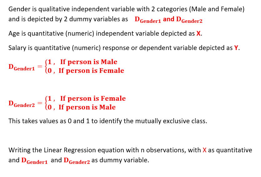
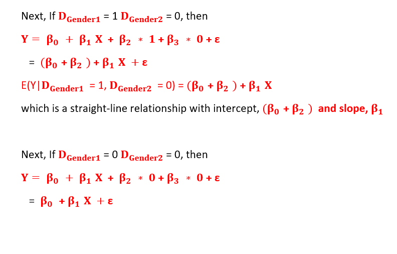
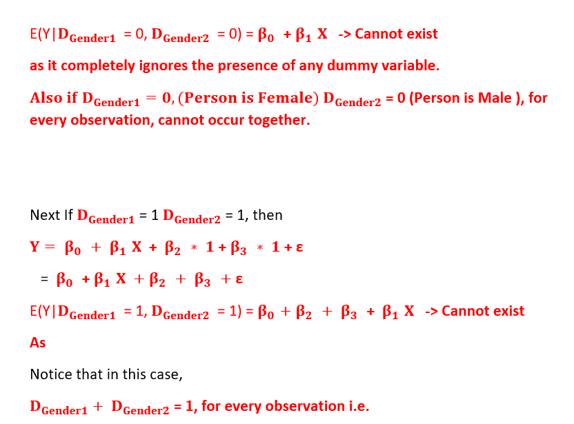
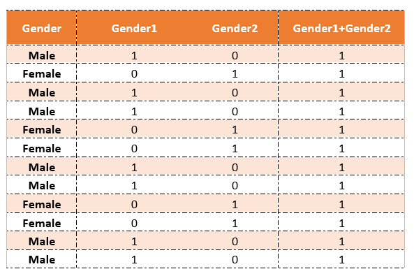
These cannot coexist together as 1 has to be 0 and the other has to be 1 to satisfy the condition, both cannot be 1 together.

The below table depicts the values.

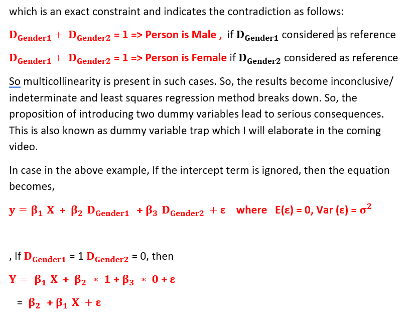
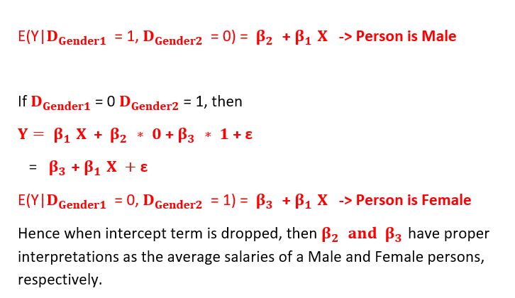
The parameters can be estimated using the ordinary least squares principle and standard procedures for drawing inferences are used.

Graphically, it looks like the below figure. It describes two parallel regression lines with the same variances.

Two parallel lines suggest the absence of any significant interaction amongst independent variables i.e., the effect of the dummy explanatory variable, Gender on the response variable, i.e., salary is the same at different values of the other explanatory variable i.e. age.

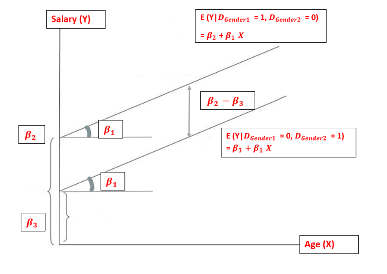
Rule: When the explanatory variable leads to m mutually exclusive categories classification, then use (m — 1) dummy variables for its representation. Alternatively, use dummy variables but drop the intercept term.

Let’s start off with our 3rd case :

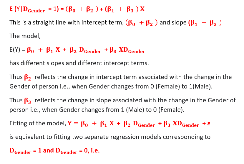
I will consider the same example as above but now I consider a situation where we have 2 independent variables with one quantitative variable and the other qualitative variable with 2 categories (Male and Female) and both of them interact and another explanatory variable as the interaction of them is added in the equation.1 dummy variable for the qualitative variable is considered.

All other things remain the same.

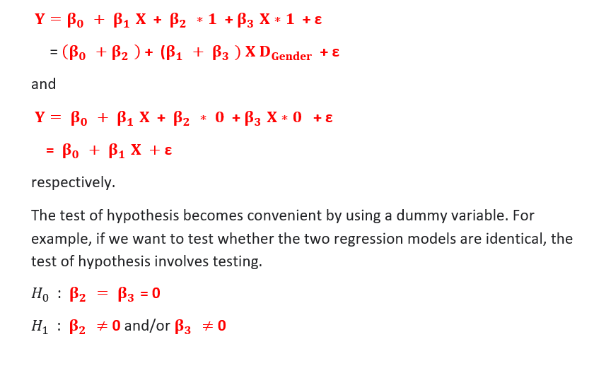
Acceptance of H0 indicates that only a single model is necessary to explain the relationship. In another example, if the objective is to test that the two models differ with respect to intercepts only and they have the same slopes, then the test of the hypothesis involves testing.

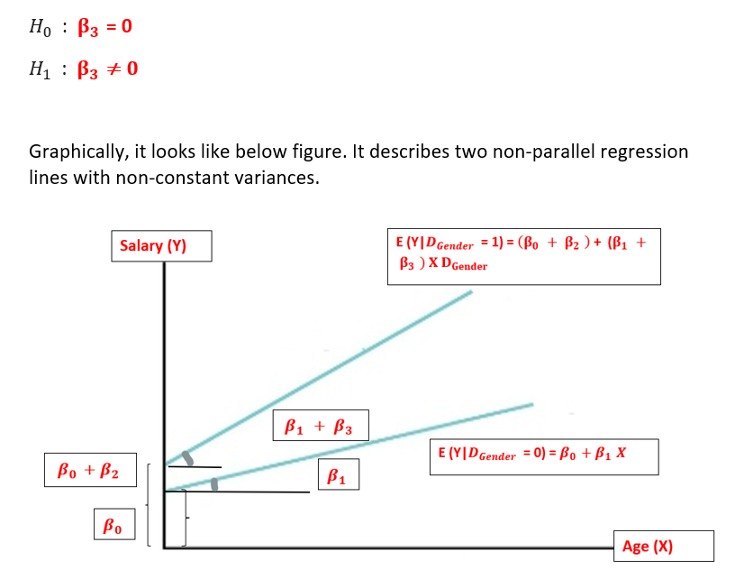
Two non-parallel lines suggest the presence of interaction amongst independent variables i.e., the effect of the dummy explanatory variable, Gender on the response variable, i.e., salary is different at different values of the other explanatory variable i.e., age.

This is a very important conclusion in itself as it affects the model significantly and as the interaction effects exist, it makes the model more complex in terms of results interpretation. We need to carefully examine linear regression results to draw insights that are because of independent variables interacting with each other.

Interaction effects in general indicate that a third variable influences the relationship between an independent and dependent variable.

As all of you know If you’re working with qualitative variables having categories, you’ll probably need to encode them to a numerical format that is more friendly to machine learning algorithms for computations. Here we make use of the method called one-hot encoding.

So, what is one-hot encoding?

One-hot encoding is the process of converting a qualitative variable with multiple categories into multiple binarized variables where each can be represented with a value of 1 or 0 to indicate the presence or absence of a class (i.e., level).

Let me show you an example through R of how it is done.

Please install the “dummies” package if not installed and then call the package using the library function.

Consider an example data with 3 columns, Salary_ per_month, Age_in_years, and Marital status.

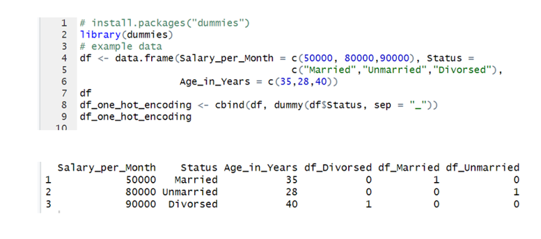
One hot encoding

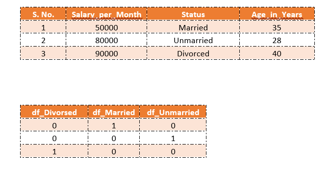
What we get here after doing one-hot encoding are dummy variables.

But one hot encoding generates as many dummy variables as there are categories in the qualitative variable i.e., if there are m categories in your one qualitative variable, it will generate m dummy variables.

We can also use the “caret” or “mltools “ package in R to do One hot encoding. So there are multiple ways in R through which you can generate dummy variables. I have considered one of the ways amongst them.

This is a case of multi-collinearity.

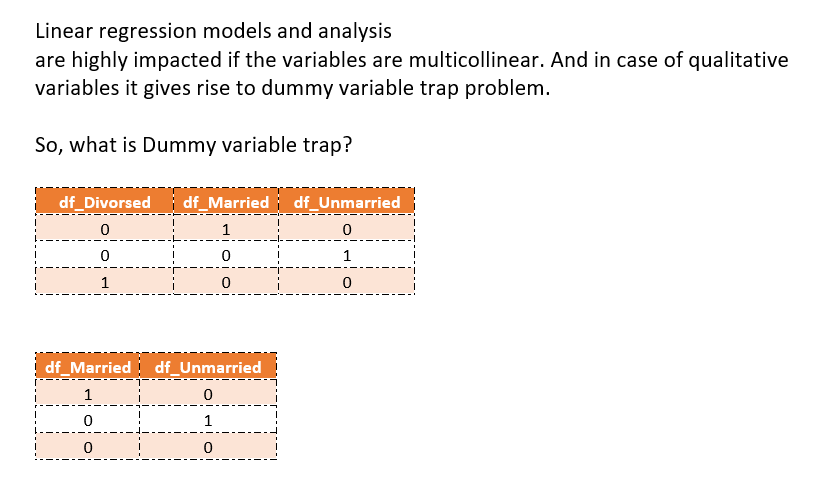
The Dummy Variable trap is a scenario in which one or several independent variables in linear regression predict another and is called multi-collinearity.

As a result, the model cannot distinguish between the effects of one column on another column.

The Dummy Variable trap is a scenario in which the independent variables are multi-collinear— a scenario in which two or more variables are highly correlated; in simple terms, one variable can be predicted from the others.

As in our case, if we know the value of variables in the 2 columns out of 3 for every observation, we can easily predict the value of the 3rd variable.

So, what is the solution in this case?

we can drop one of the dummy variables, hence removing collinearity between the added dummy variables.

There is no set rule to decide which variable can be dropped. But many software automatically sets the reference variable and drops one of the dummy variables according to the alphabetical order.

For. e.g., in our case, considering variables, df_Divorsed, df_Married, and df_Unmarried, df_Divorsed divorced will be set as reference variable and dropped off from the list as per alphabetical convention followed by software.

So, if there are m number of categories, we use m-1 variables in the model, the value of left out category can be thought of as the reference value and the remaining categories' values are fitted to represent the change from this reference.

With this, I conclude on the Dummy Variables. Though this write-up is lengthy it will definitely help to make your understanding better regarding dummy variables and their use.

Thanks for reading!!!

---

Understanding every bit of Dummy Variables — Must for AI and ML engineers was originally published in Towards AI on Medium, where people are continuing the conversation by highlighting and responding to this story.

Join thousands of data leaders on the AI newsletter. It’s free, we don’t spam, and we never share your email address. Keep up to date with the latest work in AI. From research to projects and ideas. If you are building an AI startup, an AI-related product, or a service, we invite you to consider becoming a sponsor.

Published via Towards AI