Transformers for Multi-Regression — [PART1]

Author(s): Zeineb Ghrib

Originally published on Towards AI the World’s Leading AI and Technology News and Media Company. If you are building an AI-related product or service, we invite you to consider becoming an AI sponsor. At Towards AI, we help scale AI and technology startups. Let us help you unleash your technology to the masses.

💎Transformers as Feature Extractor 💎

The FB3 competition that I joined in Kaggle has motivated me to write a post about the approaches that I tested out. Plus, I didn’t find any clear tutorial about how to use transformers for multiple regression problems, so I thought it would be useful to share my work.

All this work is resumed in my Kaggle notebook

Introduction

We don’t all have the talent of Flaubert🧡, nor the clarity of Bergson🤎, nor the genius of Proust💙, nor the style and finesse of Zweig💜, nor the skill of Voltaire💚, nor the clairvoyance of Schopenhauer💖…

And the list is far from being exhaustive, and thank God that there are writers and philosophers of genius that allow us to escape for a few moments from this materialist world.

But as far as we common people are concerned, literary or not, we can hope at least to do our best to respect the rules of the language and write “correctly”. The teachers have helped us to learn the basics of the language, so why not, in our turn we would, help them, using our knowledge, to save time to correct the essays of their students, helping them to distinguish the strong and weak points of each of their students and better adapt their pedagogy to the level of each one.

In this competition, we are asked to create an efficient model using the pre-scored argumentative essays written by 8th-12th grade English Language Learners based on six analysis metrics: cohesion, syntax, vocabulary, phraseology, grammar, and conventions. The scores range from 1.0 to 5.0 in increments of 0.5.

We will describe how to use a hugging-face model to address this type of problem, I chose deberta-v3-base model (here is the corresponding model card), and I will show how we can use it in two efficient ways:

🤙 Feature extraction: We use the hidden states as features and just train a classifier on them without modifying the pre-trained model. For this section @cdeotte proposed a brilliant use with this method consisting in using multiple non-finetuned transformers embeddings, then concatenating them and training a standalone classifier: I strongly invite you to see the related discussion and notebook

🤙 Fine-tuning: We train the whole model end-to-end, which also means updating the parameters of the pre-trained model. This approach will be discussed in a later post

In this part, we will go through the first approach step by step:👐 Introduction to the encoder-based transformer

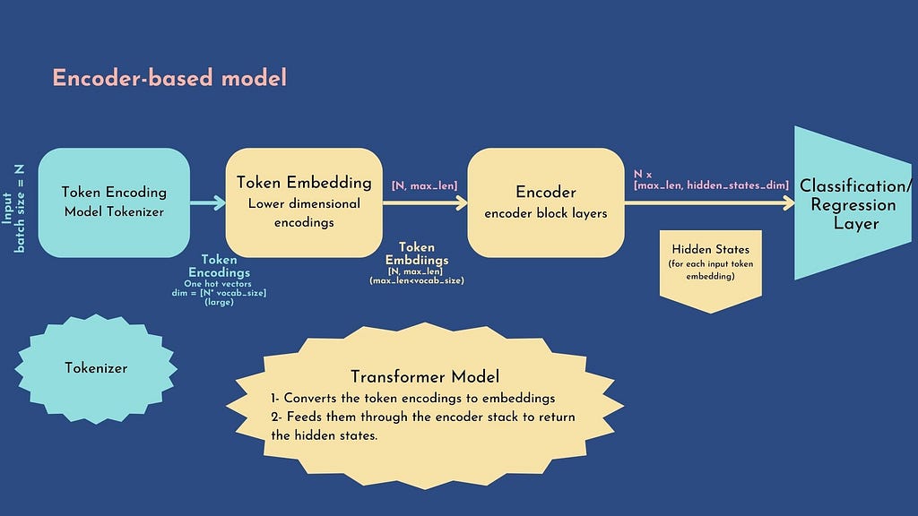
The idea is to use BERT-based models, which are pretrained to predict masked elements of texts, along with a custom classifier: the workflow is the following:

1. Generate token encoding:
First, the tokenizer generates one hot encoding called token encoding: each vector has a dimension equal to the tokenizer vocabulary [batch_size, vocab_size] . The AutoTokenizerclass of HuggingFace will automatically load the tokenizer corresponding to the checkpoint name (for this notebook, we will use deberta-v3-base), the tokenizer would generate a dictionary composed of:

• input_ids : the indices corresponding to each token in the sentence
• token_type_ids: identifies which sequence a token belongs to when there is more than one sequence
• attention_mask: identifies the padded elements from real tokens

Then the model would take the token encodings and proceed as follows:

2. Generate embeddings:
The model converts the token encodings to dense embeddings. Unlike the token encodings, the embeddings are dense= non-zero values. The token encodings are generated with the tokenizer.
-> We get a tensor with dimensions [batch_size, max_len] with the model’s maximum context size

3. Generate hidden states:
The model feeds the embeddings through the encoder stack to return the hidden states for each token input. we obtain a final tensor [batch_size, max_len, hidden_states_dim]
We load an AutoModel object to initialize a model with all the weights of the checkpoint ( microsoft/deberta-v3-base in our case)

Let's see now how to prepare our dataset to be processed by the transformer:

🪵 Prepare Dataset

We will proceed by mini-batch, and for that, we will use the torch.utils.data.DataLoader and torch.utils.data.Dataset (you can check the reference here). The Dataset allows returning the dataset samples with their corresponding labels. The DataLoader wraps an iterable around the Dataset to enable easy access to the samples, offering many utilities such as reshuffling the data at every epoch to reduce model overfitting or allowing the use of multiprocessing to speed up data retrieval.

To develop our custom Datasetwe have to override __init__ , __len__ and __getitem__ functions.
The most important function is __getitem__: it returns a sample from the dataset at a given index idx. The output format of the function must respect the expected format of the model :

• input_ids : List of token ids to be fed to the model.
• attention_mask: List of indices specifying which tokens should be attended to by the model
• labels: In our case, we deal with a multi-class regression problem, the label is a vector of the six analytics scores.

For the training method, we will refer to the undeniable classic cross-validation scheme

🍕Multi-label data stratification:

In our community of data scientists, it is evidence that the way how to split cross-validation folds has a direct impact on the model performance.
Usually, for a one-class problem, the folds are stratified along with the single target (class distribution in case of a discrete target or bins distribution for a continuous target).

But–what do we do in the case of the multi-class problem as our case🤔?

Well, many works have been carried out to deal with this problem, for example:

• 2011 : Sechidis — On the stratification of multi-label data
• 2017 : Szymański — Proceedings of the First International Workshop on Learning with Imbalanced Domains

Here is a gentle presentation to explain the algorithm.
We will use the iterative approach algorithm using the iterative-stratification implementation:

import pandas as pd
from iterstrat.ml_stratifiers import MultilabelStratifiedKFoldtrain = pd.read_csv(PATH_TO_TRAIN)
print("TRAIN SHAPE", train.shape)
test = pd.read_csv(PATH_TO_TEST)
print("TEST SHAPE", test.shape)
label_cols = ['cohesion', 'syntax', 'vocabulary', 'phraseology', 'grammar', 'conventions']
cv = MultilabelStratifiedKFold(
          n_splits=N_FOLDS, 
          shuffle=True, 
          random_state=SEED
          )
train = train.reset_index(drop=True)
for fold, ( _, val_idx) in enumerate(cv.split(X=train, y=train[label_cols])):
    train.loc[val_idx , "fold"] = int(fold)
    
train["fold"] = train["fold"].astype(int)

Now let’s implement the dataset iterator as described previously:

# lets define the batch genetator
class CustomIterator(torch.utils.data.Dataset):
    def __init__(self, df, tokenizer, labels=CONFIG['label_cols'], is_train=True):
        self.df = df
        self.tokenizer = tokenizer
        self.max_seq_length = CONFIG["max_length"]# tokenizer.model_max_length
        self.labels = labels
        self.is_train = is_train
        
    def __getitem__(self,idx):
        tokens = self.tokenizer(
                    self.df.loc[idx, 'full_text'],#.to_list(),
                    add_special_tokens=True,
                    padding='max_length',
                    max_length=self.max_seq_length,
                    truncation=True,
                    return_tensors='pt',
                    return_attention_mask=True
                )     
        res = {
            'input_ids': tokens['input_ids'].to(CONFIG.get('device')).squeeze(),
            'attention_mask': tokens['attention_mask'].to(CONFIG.get('device')).squeeze()
        }
        
        if self.is_train:
            res["labels"] = torch.tensor(
                self.df.loc[idx, self.labels].to_list(), 
            ).to(CONFIG.get('device')) 
            
        return res
    
    def __len__(self):
        return len(self.df)

This custom Dataset will be used later either to fine-tune the transformer or just use it as a feature extractor.

PS: I added the is_train parameter to whether return the “labels” field or not (only the training dataset contains the labels field)

⛏Transformers as Feature Extractors⛏

With this method, the encoder weights are frozen, and the hidden states are used as standalone features by the multi-regressor.
Since the hidden states are computed once, this method is the best choice if we do not dispose of GPUs :

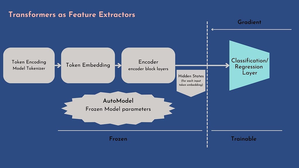
The only axe of freedom that remains to us is how to reduce the hidden states tensor [batch_size, max_len, hidden_states_dim] to a single vector representation: I urge you to consult the invaluable @rhtsingh notebook that enumerates “exhaustively” the different ways to ”pool” the hidden states encodings.

I tested out the following techniques:

🤙 CLS embedding: BERT introduces a [CLS] token tag standing in the first position of each sentence that captures the whole sentence context. The cls embedding simply consists in selecting the first element of each hidden state vector, to get down to [batch_size, 1, hidden_states_dim] vector

import torch
import torch.nn as nn
import transformers
from transformers import (
    AutoModel, AutoConfig, 
    AutoTokenizer, logging,
    AdamW, get_linear_schedule_with_warmup,
    DataCollatorWithPadding,
    Trainer, TrainingArguments
)
from transformers.modeling_outputs import SequenceClassifierOutput# https://github.com/UKPLab/sentence-transformers/blob/0422a5e07a5a998948721dea435235b342a9f610/sentence_transformers/models/Pooling.py
# https://www.kaggle.com/code/rhtsingh/utilizing-transformer-representations-efficiently
def cls_embedding(outputs):
    """Since Transformers are contextual model, 
    the idea is [CLS] token would have captured the entire context 
    and would be sufficient for simple downstream tasks such as classification
    Select the first token for each hidden state
    
    @param outputs: the model output dim = [batch_size, max_len, hidden_states_dim]
    @return:  tensor of dimensions = [batch_size, hidden_states_dim]
    """
    return outputs.last_hidden_state[:, 0, :].to(CONFIG.get('device'))

🤙 Mean pooling: rather than selecting the first element we will consider the average of max_len dimensional embeddings for each hidden state dimension: we obtain a tensor of[batch_size, 1, hidden_states_dim] or just the unsqueezed form : [batch_size, hidden_states_dim]

def mean_pooling(inputs, outputs):
    """
    For each hidden_state, average along with max_len embeddings, 
    but we will condider only the highlighted tokens by the attention mask
    
    @param inputs: = the tokenizer output = the model input : a dict must contain at least the attention_mask field
    @param outputs: the model output dim = [batch_size, max_len, hidden_states_dim]
    @return:  tensor of dimensions = [batch_size, hidden_states_dim]
    """
    input_mask_expanded = inputs['attention_mask'].squeeze().unsqueeze(-1).expand(outputs.last_hidden_state.size()).float()
    sum_embeddings = torch.sum(outputs.last_hidden_state * input_mask_expanded, 1)
    sum_mask = input_mask_expanded.sum(1)
    sum_mask = torch.clamp(sum_mask, min=1e-9)
    mean_embeddings = sum_embeddings / sum_mask
    return mean_embeddings

🤙 Max Pooling: to get the max pooling we will take the max across max_len embeddings at each hidden state dimension, the result is a tensor of [batch_size, hidden_states_dim] dimensions

def max_pooling(inputs, outputs):
    """
    For each hidden_state, get the max element along with max_len embeddings,
    considering only the non masked element difined by the attention mask computed by the tokenizer
    
    @param inputs: = the tokenizer output = the model input : a dict must contain at least the attention_mask field
    @param outputs: the model output dim = [batch_size, max_len, hidden_states_dim]
    @return:  tensor of dimensions = [batch_size, hidden_states_dim]
    
    """
    last_hidden_state = outputs.last_hidden_state
    input_mask_expanded = inputs['attention_mask'].squeeze().unsqueeze(-1).expand(outputs.last_hidden_state.size()).float()
    last_hidden_state[input_mask_expanded == 0] = -1e9  # Set padding tokens to large negative value
    max_embeddings = torch.max(last_hidden_state, 1).values
    return max_embeddings

🤙 Mean-Max Pooling: we apply the mean pooling and the max pooling, then concatenate the two to get[batch_size, 2*hidden_states_dim] dimensional tensor

def mean_max_pooling(inputs, outputs):
    """
    Apply mean and max-pooling embeddings, then we concatenate the two onto a single final representation
    
    @param outputs: the model output dim = [batch_size, max_len, hidden_states_dim]
    @return:  tensor of dimensions = [batch_size, 2*hidden_states_dim]
    """
    mean_pooling_embeddings = mean_pooling(inputs, outputs)
    max_pooling_embeddings = max_pooling(inputs, outputs)
    mean_max_embeddings = torch.cat((mean_pooling_embeddings, max_pooling_embeddings), 1)
    return mean_max_embeddings

Here a code sample to get all the embeddings:

def get_embedding(dataloader, model, n):
    """
    Run the model to predict hidden states then apply all the transformations implemented above
    
    @param dataloader: a torch.utils.data.DataLoader the iterator along with the custom torch.utils.data.Dataset
    @param model : the huggingface AutoModel that generates the hidden states
    """
    embeddings = {}
    model = model.to(CONFIG.get('device'))
    for batch in tqdm_notebook(dataloader):
        with torch.no_grad():
            # please note here that the labels fileds is not necessary 
            # since we are not going to fine tune the model but just get the vectors output
            outputs = model(
                input_ids=batch['input_ids'].squeeze(),
                attention_mask=batch['attention_mask'].squeeze()
            )
        for embed_name, embed_func in zip(['cls_embeddings', "mean_pooling", "max_pooling", "mean_max_pooling"], 
                                          [cls_embedding, mean_pooling, max_pooling, mean_max_pooling]):
            if embed_name == 'cls_embeddings':
                embed = embed_func(outputs)
            else:
                embed = embed_func(batch, outputs)
            embeddings[embed_name] = torch.cat(
                (
                    embeddings.get(embed_name, torch.empty(embed.size()).to(CONFIG.get('device'))), 
                    embed
                ),
                0
            )
    threshold = min(n,CONFIG.get('train_batch_size'))
    for key in embeddings:
        embeddings[key] = embeddings[key][threshold:,:]
    return embeddings

Now let’s see how to generate the embeddings for both train and test datasets:

model = AutoModel.from_pretrained(CONFIG["model_name"], config=config)
# TRAIN #
df_iter = CustomIterator(train, tokenizer)
train_dataloader = torch.utils.data.DataLoader(
    df_iter, 
    batch_size=CONFIG["train_batch_size"],
    shuffle=False
)
embeddings = get_embedding(train_dataloader, model, n=len(train))
# TEST #
df_iter = CustomIterator(test, tokenizer, is_train=False)
test_dataloader = torch.utils.data.DataLoader(
    df_iter, 
    batch_size=CONFIG["train_batch_size"],
    shuffle=False
)
test_embeddings = get_embedding(test_dataloader, model, n=len(test))

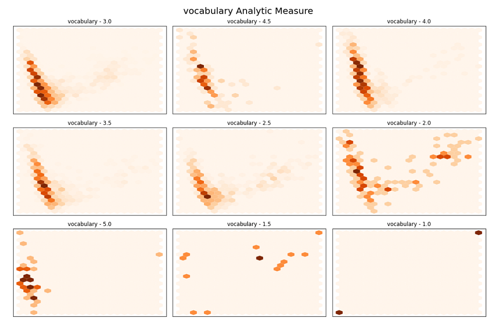
🔍 Hidden States visualization:

Let’s take a look at the embeddings before training a classifier to get 2D visualization. For simplicity, we will apply it only for the cls_embeddings it would be the same for the other types of embeddings.

We have to reduce the hidden states to 2D, many efficient models can be used to reduce the dimensions of the embeddings: UMAP, PCA, T-SNE

We will use the PCA algorithm:
1. Data normalization: Standardize the embeddings using StandardScaler of scikit learn
2. 2D dimension reduction: fit a PCA model on the embeddings and extract the two first components
3. Hexbin Visualization: for each target class, we will visualize the bins of each score (from 1 to 5 with step = 0.5)

Let’s take a look at the Vocabulary class plot:

PS: This visualization section technique is very inspired by this HuggingFace NLP GitHub example

Some patterns can be identified from this plot, : for most of them, extreme scores are well separated, 2.5 scores seem to be scattered around all places, and for the others, there are clear overlaps.

PS: Do not forget that these embeddings are generated by a model pre-trained on predicting masked words in sentences, not to classify scores.

⚙ Multi-Regressor Head Training

Let’s train a multi-regression model on our embeddings: I chose a gradient boosting-based model: Xgboost

In our case: multi-class regression, we will be using the MultiOutputRegressor estimator of scikit-learn. I will let you check the original and further implementation from @SWIMMY excellent notebook of different tree-based models + stacking with a meta-model.

To see which pooling has the best separation representation, we will use the cross-validation evaluation for each pooling embedding. The global metric consists of averaging the RMSEs of the 6 of the target columns: this metric is called MCRMSE (mean column-wise root mean squared error)

Let’s define the evaluation metric:

def comp_score(y_true,y_pred):
    rmse_scores = []
    for i in range(len(CONFIG['label_cols'])):
        rmse_scores.append(np.sqrt(mean_squared_error(y_true[:,i],y_pred[:,i])))
    return np.mean(rmse_scores)

Now launch the CV training:

import joblib
y_true = train[CONFIG['label_cols']].values
cv_rmse = pd.DataFrame(0, index=range(N_FOLDS), columns=embeddings.keys())

oof_pred = {
        emb_type : np.zeros((len(train), len(label_cols)))
        for emb_type in embeddings
    }

for emb_type, emb in embeddings.items(): 
    print(f"CV for {emb_type}")
    emb = normalize(
        emb, 
        p=1.0, 
        dim = 1
    ).cpu()

    for fold, val_fold in train.groupby('fold'):
        print(f"*** FOLD == {fold} **")
        x_train, x_val = np.delete(emb, val_fold.index, axis=0), emb[val_fold.index]
        y_train, y_val = np.delete(y_true, val_fold.index, axis=0), y_true[val_fold.index]
        xgb_estimator = xgb.XGBRegressor(
                n_estimators=500, random_state=0, 
                objective='reg:squarederror')
        # create MultiOutputClassifier instance with XGBoost model inside
        xgb_model = MultiOutputRegressor(xgb_estimator, n_jobs=2)
        # model4 = XGBClassifier(early_stopping_rounds=10)
        xgb_model.fit(x_train, y_train)
        oof_pred[emb_type][val_fold.index] = xgb_model.predict(x_val)
        for i, col in enumerate(CONFIG['label_cols']):
            rmse_fold = np.sqrt(mean_squared_error(y_val[:,i], oof_pred[emb_type][val_fold.index,i]))
            print(f'{col} RMSE = {rmse_fold:.3f}')
            
        cv_rmse.loc[fold, emb_type] = comp_score(y_val, oof_pred[emb_type][val_fold.index])
        print(f'COMP METRIC = {cv_rmse.loc[fold, emb_type]:.3f}')        
        joblib.dump(xgb_model, f'xgb_{emb_type}_{fold}.pkl')

During the CV training, for each embedding type, a fold is kept apart at each iteration, and the model is trained on the remaining fold. Then we predict the unseen fold. Hence we obtain out-of-fold predictions (OOF predictions), which means that every prediction has been accomplished on unseen data.

Then we evaluate the RMSE on each class and the global MCRMSE on the OOF predictions for each embedding type: we obtain the following performances:

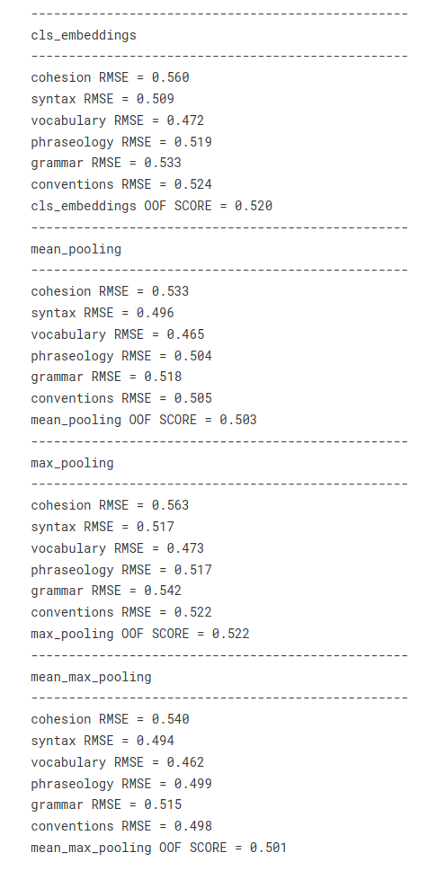
• It seems like the MeanMax pooling gives the best performance, but the Mean pooling is veeery close. As the mean max pooling takes twice the volume as the mean pooling, we will choose the mean encoding to fine-tune the transformer
• The least efficient pooling method on our corpus is the Max pooling
• For all of the representations of analysis metrics, vocabulary is the easiest target to estimate (lowest RMSE), and cohesion is the hardest one (highest RMSE)

To infer new predictions, a friend of mine, Mathurin Aché, who is also a great data scientist and a Kaggle master, taught me two methods :

1. Use the CV models to predict the new data: averaging the predictions allows for reduce variance however increases the prediction per sample time, and if we have to deploy this approach, we have to save all the CV models
2. Train the retained model on the whole training data once, then predict the new predictions, which can increase a little the generalization error a, but it is recommended in case of deployment (prediction time and single model to monitor)

As long as we are in Kaggle competition context we opted for the first method, using the Mean-Max Pooling:

import glob
# init output with zeros
xgb_infer = np.zeros((len(test), len(label_cols)))
for model_path in glob.glob("./xgb_mean_max_pooling_*.pkl"):
    print(f"load {model_path} model")
    xgb_model = joblib.load(model_path)
    emb = normalize(
        test_embeddings["mean_max_pooling"], 
        p=1.0, 
        dim = 1
    ).cpu()
    # add fold model prediction
    xgb_infer = np.add(xgb_infer, xgb_model.predict(emb))
# devide by the number of folds
xgb_infer = xgb_infer*(1/N_FOLDS)

🙏Credits:

My work in this part was inspired by these excellent resources, do not hesitate to consult them:

• @swimmy notebook: an excellent recap for gradient boosting models blending, I borrowed the XGBoost part that I applied to the transformer embedding
• @rhtsingh notebook: the different ways to explore transformer representations
• @Y.NAKAMA notebook: the loss function and the multilabel — Stratified cross-validation
• Huggingface NLP GitHub: the dimension reduction and the transformer embedding visualization

Conclusion:

Thanks for Reading my post 🤗I hope it will be useful! As a reminder, all my work can be found here🎁.

In this post, we saw how to use a pre-trained transformer to extract context-capturing embeddings and use it to train a multi-regressor (Xgboost in our case) to model analysis metrics of the student's essays.

In the next part, I will address the same problem but by fine-tuning the transformer, and updating all its encoder stack, this time. Furthermore, I will show you how to use Weights & Biases great platform to track model performances and create model artifacts. Transformers for Multi-Regression task

---

Transformers for Multi-Regression — [PART1] was originally published in Towards AI on Medium, where people are continuing the conversation by highlighting and responding to this story.

Join thousands of data leaders on the AI newsletter. It’s free, we don’t spam, and we never share your email address. Keep up to date with the latest work in AI. From research to projects and ideas. If you are building an AI startup, an AI-related product, or a service, we invite you to consider becoming a sponsor.

Published via Towards AI