The intuition behind the Central Limit Theorem

Last Updated on January 6, 2023 by Editorial Team

Author(s): Alison Yuhan Yao

Statistics

The easiest example for intuition & CLT visualized in Python

All visualization code and calculation for mean and sd are in this GitHub notebook.

The Central Limit Theorem (CLT) is one of the most important and most beautiful theorems in Statistics and Data Science. In this blog, I will explain a simple and intuitive example about the distribution of the means and visualize CLT using python.

Let’s start from the basics.

Distribution of Means vs Distribution of Scores

When we talk about statistics, most people think about the distribution of scores. That is, if we have 6, 34, 11, 98, 52, 34, 13, 4, 48, 68, we can calculate the mean of the 10 scores:

and subsequently, the population standard deviation is:

The distribution of means, on the other hand, looks at groups of 2 or 3 or more scores in a sample. For example, if we group the scores out of convenience, we can have 6 and 34 as group 1, 11 and 98 as group 2, and so on. We look at the mean of all the groups, which are (6+34)/2=10, (11+98)/2 = 54.5, etc. And then, we calculate the mean of the distribution of 5 means, which should be the same as the mean of the distribution of scores 36.8.

Therefore, you can imagine the distribution of scores as studying 6, 34, 11, 98, 52, 34, 13, 4, 48, 68 (the 10 scores) and the distribution of means as studying 10, 54.5, 43, 8.5, 58 (the 5 means).

But of course, this type of grouping 2 scores is only for demonstration’s sake. In reality, we bootstrap (random sampling with replacement) from the 10 scores and have an infinite number of groups of the same size N.

Next, let’s dive into a simple coin example.

CLT visualized with example

Misunderstanding of CLT

Suppose we have 1000 fair coins and we denote head as 1 and tail as 0. If I flip each coin once, we will ideally get a distribution like this:

I emphasize ideally because in reality, one might easily end up with a 501/499 or 490/510 split.

So why is 500/500 ideal? It seems quite easy to understand this intuitively. How can we prove this mathematically?

To answer that, we need to talk a little about probability.

Probability deals with predicting the likelihood of future events, while statistics involves the analysis of the frequency of past events. [1]

Before that, we have been talking strictly about statistics because we are looking at experiment results and counting heads and tails. However, when foreseeing an ideal case where heads and tails are equally split, we are predicting the likelihood of what is supposed to happen when the sample size is very large. And what’s supposed to happen is consistent with the probability of something happening thanks to the Law of Large Numbers. Please note that to use LLG, the sample size needs to be infinitely big.

To illustrate, let’s do another experiment with fair coins, but this time we have 100000000000 of them. What do you expect to happen? Again, we will ideally get a distribution like this:

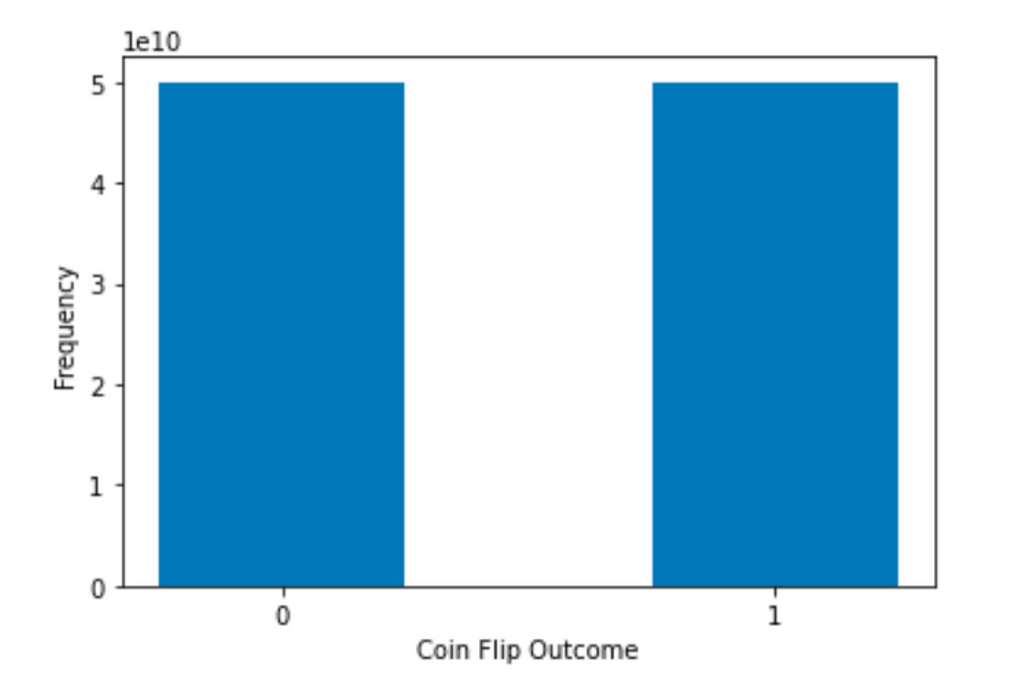
That’s because, for a fair coin, the probability of tossing a head or a tail is the same, which are both 0.5. So we would expect the actual outcome to be closer to half-half when the sample size is much larger.

Another very important point here is that increasing the samples size does not change the shape of the distribution of scores!

No matter how many fair coins one tosses, the outcome will never become a normal distribution because CLT is about the distribution of means, not the distribution of scores.

We can easily calculate the mean and standard deviation according to the distribution of infinite scores. When we toss n fair coins (n goes to infinity), we will have n/2 heads and n/2 tails.

CLT Visualized

Now, we take a look at the means of pairs of coins, meaning that we group 2 coins together and have an infinite number of groups of 2 coins. The possible means of 2 coins are 0, 0.5, and 1.

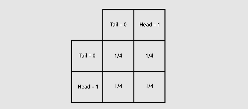
The probability of the first coin to be tail and the second coin to be tail is 1/2 * 1/2 = 1/4. As are the other three.

Therefore, the probability to get a mean of 0 (both tails) is 1/4. The probability of getting a mean of 0.5 (one tail and one head) is 1/4 * 2= 1/2. The probability to get a mean of 1 (both heads) is also 1/4.

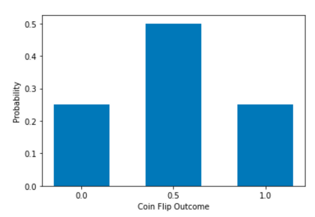
Then, the distribution would look like this. Please note that the y-axis is now Probability instead of Frequency (aka count), but the shape is the same no matter which y-axis you use. Compared to the previous bar chart, we now have 3 bars with a peak in the middle.

Again, we calculate the mean and standard deviation:

The mean stays the same, but the sd is smaller now.

Similarly, we can group 3 coins together. The possible means of 3 coins are now 0, 1/3, 2/3, and 1. There are 2 * 2 * 2 = 8 combinations in total.

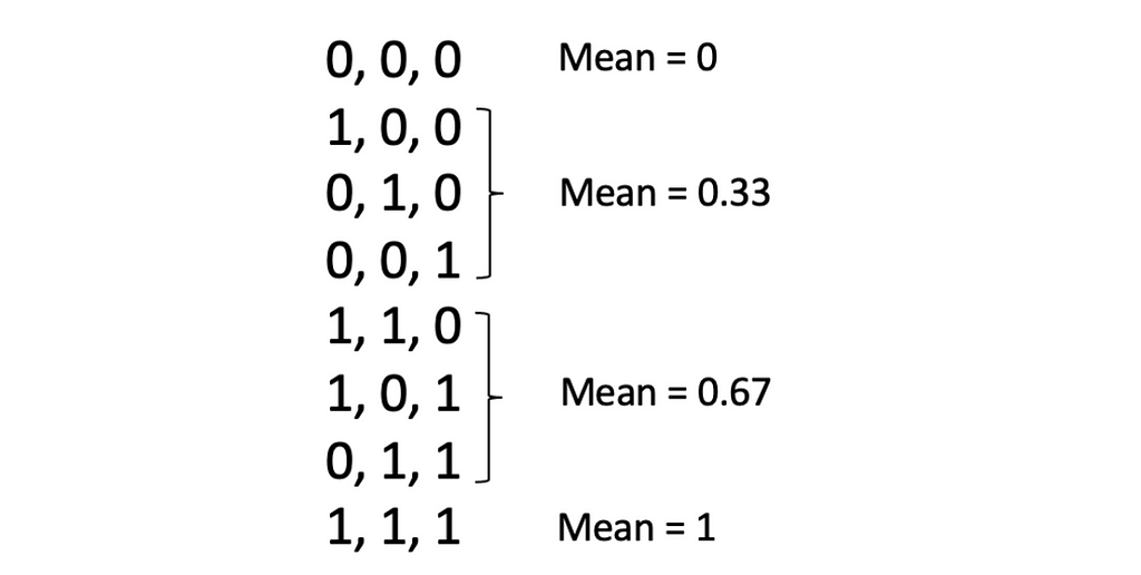
Probability of getting a mean of 0 is p(0) = 1/8.

Similarly,
p(0.33) = p(0.67) = 3/8 and
p(1) = 1/8.

The mean and standard deviation are:

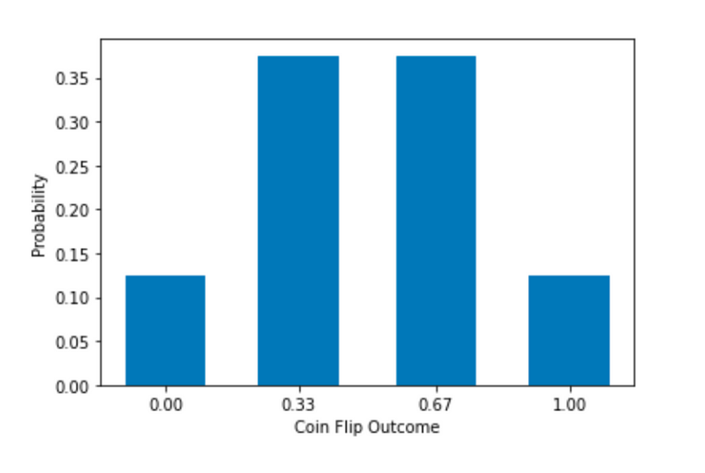
The distribution now has 4 bars, 1 more than the previous one, again. The mean stays the same and the sd is decreasing.

That seems to be a pattern.

What will happen to the mean, standard deviation, and distribution if we were to increase the value of N?

To see if it is indeed a pattern, I calculated and visualized more results. The number N below is the number of coins in each group. The distribution of scores implies N = 1.

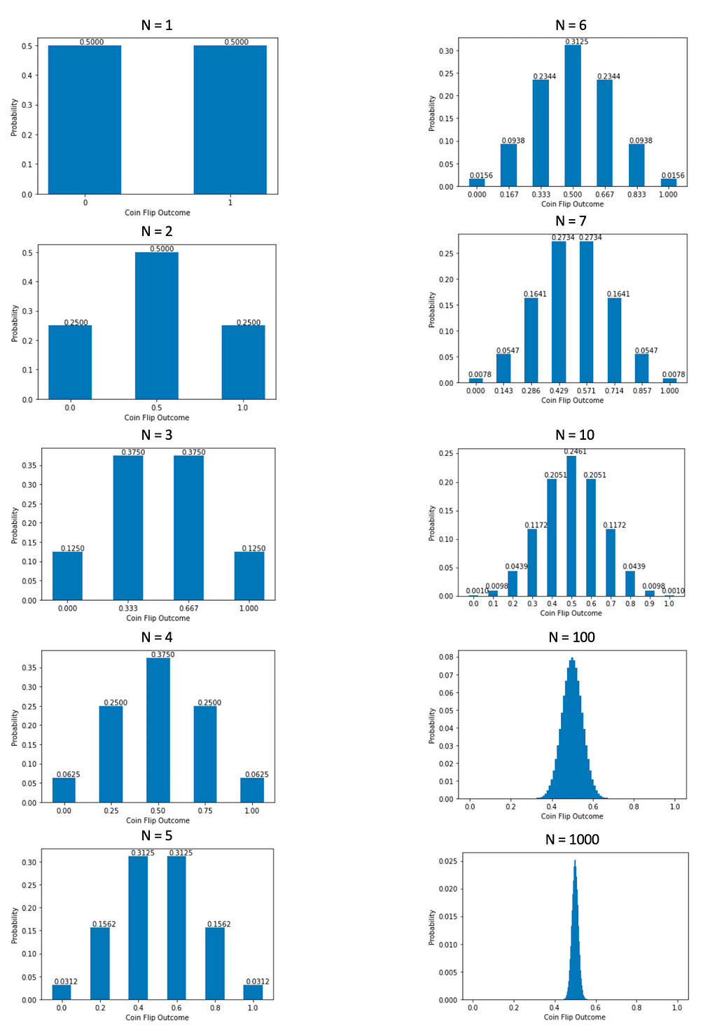
Now, it is easy to see that as N becomes bigger, the distribution of means gets closer to a bell-shaped normal distribution. When N is extremely big, we can hardly see the bars on the sides because the probabilities are too small, but the possible means still range from 0 to 1.

We can also see that the mean of the distribution of means is always 0.5, while the standard deviation of the distribution of means is continuously decreasing because the visible shape is getting narrower.

Standard Error

We actually have a way to quantify the changes in the standard deviation as N becomes larger. I wrote the following python code to calculate the mean and standard deviation.

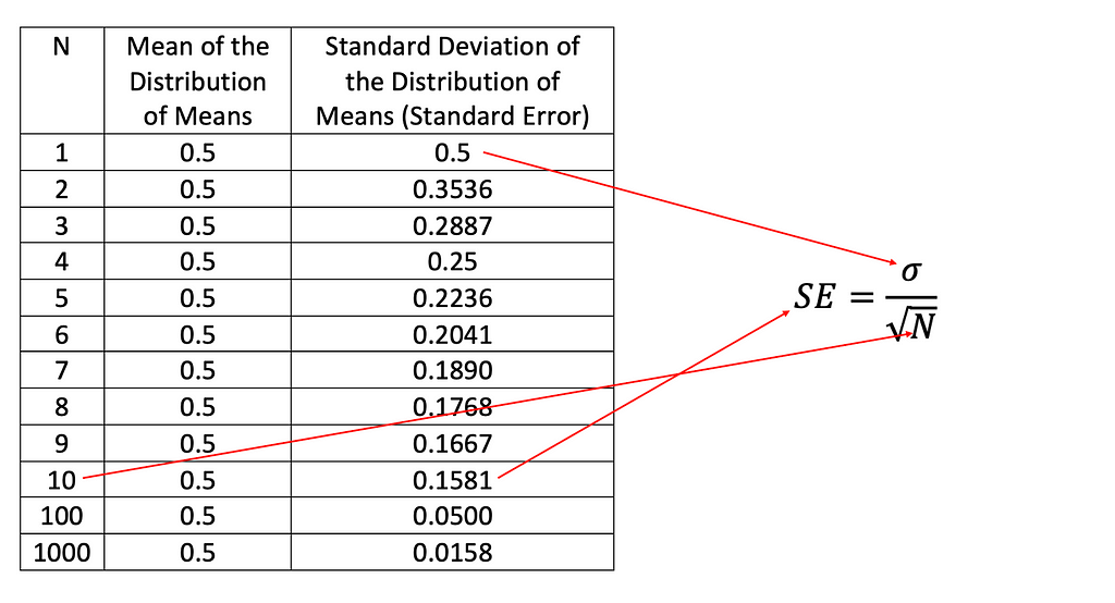
Again, we can see that the mean stays the same and the sd of the distribution of means drops as N gets larger. The standard deviation of the distribution of means is also called the standard error (SE) and the relationship between SE and N is SE = sigma/the square root of N. In this case, sigma = 0.5 because when N=1, aka when a group only has one score, it is a distribution of scores. When N is equal or greater than 2, it becomes a distribution of means. And as N increases, the denominator of SE increases, so SE decreases.

Conclusion

To wrap up, we have studied the coin example closely and learned the following points:

• The distribution of scores is different from the distribution of means.
• CLT employs the distribution of means to get a normal distribution when the number of scores to calculate a mean (N) is infinitely large. No matter how large the sample size is, the distribution of scores is not going to be normal.
• The mean of the distribution of means equals the mean of the distribution of scores.
• The standard deviation of the distribution of means, aka standard error, decreases as the number of scores to calculate a mean (N) increases. And the accurate relationship is:

All visualization code and calculation for mean and sd are in this GitHub notebook.

Thank you for reading! I hope this has been helpful to you.

Special thanks to Professor PJ Henry for introducing the coin example in class. I’ve modified it and added my own explanation and visualization here.

References

[1] Steve Skiena, “Probability versus Statistics”, Calculated Bets: Computers, Gambling, and Mathematical Modeling to Win! (2001), Cambridge University Press andMathematical Association of America

---

The intuition behind the Central Limit Theorem was originally published in Towards AI on Medium, where people are continuing the conversation by highlighting and responding to this story.

Published via Towards AI