Sound and Acoustic patterns to diagnose COVID [Part 1]

Author(s): Himanshu Pareek

Originally published on Towards AI the World’s Leading AI and Technology News and Media Company. If you are building an AI-related product or service, we invite you to consider becoming an AI sponsor. At Towards AI, we help scale AI and technology startups. Let us help you unleash your technology to the masses.

Link to Part 2 of this case study

Link to Part 3 of this case study

Understanding the problem and background

In this case study, we will attempt to build a model that could diagnose COVID using sound and audio waves. This would require us to design and build custom deep learning models that can detect small changes in speech/audio to detect the medical condition in question.

Early diagnosis of any disease is key for a successful treatment. Undiagnosed diseases cost millions of people their lives and savings every year. If we can find a cost-effective, simple way to alert a user about possible diseases they might have, it would help them seek medical counseling early and address the problems effectively. Today, we have access to large amounts of data, an arsenal of computational resources, and sufficient advances in deep learning methods that could help us solve these problems.

There is some research that shows that physiological changes and changes in biochemistry affect the sounds created by the human body. In human history, bodily noises are long used in the diagnosis of ailments. Medical research literature establishes this connection, thus becoming a foundation for the development of ML solutions over speech, sound, and acoustic data.

An ML model of high accuracy will be a cheap and faster alternative to traditional chemical-based tests and can be productionized at scale. Our aim should be to make an ecosystem of technology-driven solutions and currently popular testing methods, to effectively respond to pandemics of the future, and to improve the medical services available to people.

Dataset:

Ideally, for disease detection, we would want users to register sounds in their smart devices in the following form — cough, reading a paragraph to record speech, directed breathing sounds. This can be done actively through direction, or passively by recording through smart devices like phones, or smart assistants. Our data set will consist of cough sounds, that a user can record and test.

Cough sounds:

The core airways — bronchi and trachea — are cleared up of secreted or inhaled particles by a strong reflex mechanism called cough. In normal situations, the reflex follows a standard process from inhaling to exhaling. It is often triggered by physical and chemical inputs. Thoracic pressure is built which is released with an explosion of sound and liquid. This pressured expulsion causes movement of fluid, air turbulence, and vibration of mass, causing a distinct sound. The frequency and broadband of this sound depend on a number of factors, such as the diameter of the airway paths, density, and strength of the expelled air. The sound is a composite of 3 temporal phases — explosive, intermediate, and voicing. The frequency spectrum lies between 500 hertz to 3.8 kilohertz. This is sufficient for recording a cough sound using a microphone – a key observation for our case study. Pulmonary diseases like COVID and pneumonia change the physical structure of the respiratory tract, making it possible for us to identify them using cough sounds. There is already a lot of positive research around accurate identification of diseases like Pertussis, COPD (chronic obstructive pulmonary disease), tuberculosis, asthma, and pneumonia using cough sounds.

Real-world challenges and constraints

The data is not easy to obtain. People have to take the time to provide sound recordings and metadata about them, to create a large enough database. Also, for our solution to be relevant in the real world, the model should be trainable on a small amount of data as well, so in case of a new pandemic or a new strain of virus, we can create and deploy a solution quickly to address the problem.

We must ensure that a web app deployed for our product should be able to process the sound recordings in a reasonable time.

Also, it is absolutely critical to be able to provide accurate results to a user using our web app. False negatives will quickly destroy the credibility of the solution.

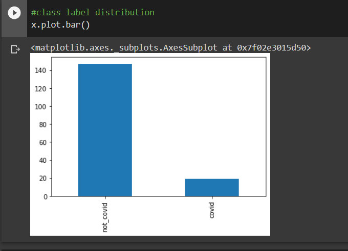
For this case study, we will use a small dataset.

The data set can be downloaded from below:

https://data.mendeley.com/datasets/ww5dfy53cw/1

#class label distribution

x.plot.bar()

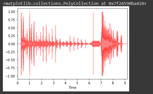
#visualise the wave file

import librosa as lb
import librosa.display

a,b = lb.load('/gdrive/MyDrive/Kaggle/trial_covid/--U7joUcTCo_ 0.000_ 10.000.wav', mono=True)

librosa.display.waveplot(y=a, sr=b, max_points=100000.0, color='r', alpha=0.5)

EDA, feature extraction, and understanding of features

Extraction of features and analyzing them is important to find relations between data points. The audio can not be directly fed to a model, so extracting features is significant. It explains the majority of information embedded in the audio signal in an explainable form. Extracting features from audio is needed for classification, regression, or clustering tasks. Time, frequency, and amplitude are 3 important dimensions of a sound signal.

The time it takes for a wave to finish one full cycle is called it's period. The number of cycles a signal does in a second is the frequency. The inverse of the frequency is the time period. The metric of frequency is hertz. A lot of sounds in nature are complex and composite of many frequencies and they can be represented as the addition of these different frequencies. Vectorizing sound is needed for machine learning and it is achieved by measuring the amplitude of sound at different times. This measurement is called a sample, and the number of samples taken per second is the sampling rate.

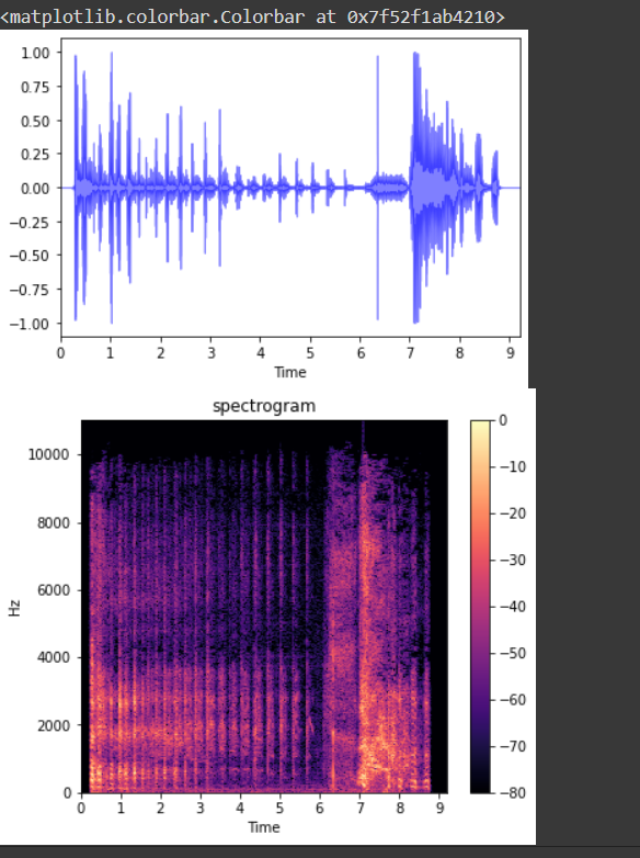
Spectrogram:

Spectrograms are visualization of audio, a method to view an audio wave in a form of an image. The frequencies embedded in an audio form the spectrum. A spectrum is a way to see sound in the frequency domain. The spectrogram has these colors, which represent a spectrum of frequencies. Each color represents the strength or amplitude of the frequency. Thus, it represents the spectrum of frequencies of an audio wave over time in the form of color bands. Lighter colors represent heavy concentrations of frequencies, while darker colors mean low to no concentrations.

Spectrograms are created by dividing the audio into time windows and taking a Fourier transform on each of the windows. Each window is converted to a decibel unit for better results.

It is interesting to note that sound is stored in memory as a series of numbers, where the numbers are amplitudes. If we take 100 samples in a second, the 1-second audio would be stored as a series of 100 numbers.

#Plot wave and its spectrogram

y,sr = librosa.load('trial_covid/--U7joUcTCo_ 0.000_ 10.000.wav', mono=True)

librosa.display.waveplot(y=y, sr=sr, max_points=100000.0, color='b', alpha=0.5)

print('\n\n')

#short time fourier transform of y, taking absolute values.

y_t = np.abs(librosa.stft(y))

#conversion to decibles

y_t_d = librosa.amplitude_to_db(y_t, ref=np.max)

#plotting

figure, ax = plt.subplots(figsize=(6,5))
spectrogram = librosa.display.specshow(y_t_d, sr=sr, y_axis='linear', x_axis='time', ax=ax )

ax.set(title='spectrogram')

figure.colorbar(spectrogram)

Zero crossing Rate:

This represents the rate of change of sign as the signal progresses. How many times a wave moves from positive to negative is captured in this feature. This is heavily used in speech recognition. Zero crossing rate is higher for percussive sounds, such as discharge of a firearm, playing a musical instrument, etc.

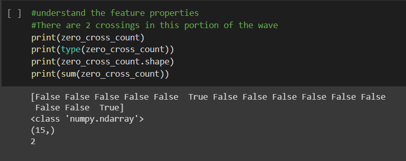
#Visualizing zero crossing

#pad false means, y[0] will not be considered as a zero crossing

y, sr = librosa.load('trial_covid/--U7joUcTCo_ 0.000_ 10.000.wav', mono=True)

#zooming into the wave
plt.plot(y[8000:8015])
zero_cross_count = librosa.zero_crossings(y[8000:8015], pad=False)

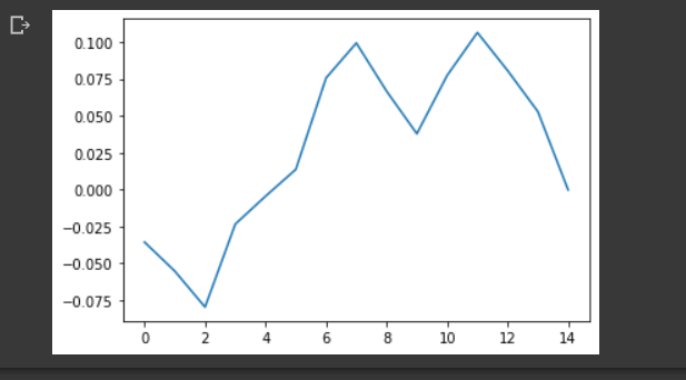
There are 2 crossings in this portion of the wave.

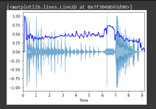
Spectral centroid:

The spectral centroid represents the center of mass of an audio signal, which is calculated using the weighted mean of all the frequencies composed in the sound. If the sound signal is uniform and has the same frequency distribution from start to end, then the centroid will be in the middle, however, if there are higher frequencies at the start than at the end, the centroid will shift to the left.

There is a rise of centroid at the beginning, because the amplitude is low there, giving high-frequency portions a chance to dominate.

# Spectral centroid
# t frames of the spectrogram will give t centroids.

import sklearn #need for normalization

spec_cent = librosa.feature.spectral_centroid(y,sr=sr)[0]

#frames for visualization

l = range(len(spec_cent))

frames = librosa.frames_to_time(l)

spec_cent_nor = sklearn.preprocessing.minmax_scale(spec_cent, axis=0)

librosa.display.waveplot(y,sr=sr,alpha=0.5)

plt.plot(frames, spec_cent_nor, color='b')

Spectral Rolloff:

Spectral roll-off is the frequency below which a certain percentage of total spectral energy lies. This is configurable. For example, at a frequency of “F”, 90 percent of spectral energy lies below F.

#spectral rolloff - similar to centroid in implementation.

spec_rolloff = librosa.feature.spectral_rolloff(y,sr=sr)[0]

spec_rolloff_nor = sklearn.preprocessing.minmax_scale(spec_rolloff, axis=0)

Mel Spectrograms:

These are spectrograms based on the mel scale instead of the hertz scale. The mel scale transforms frequency using a logarithm. The transformation is as follows:

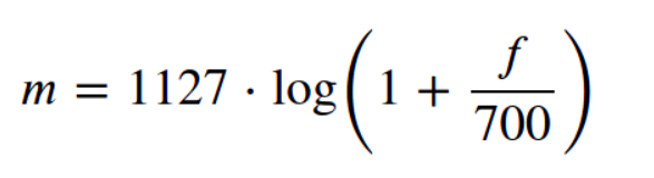
For a natural logarithm used above, the coefficient is 1127. If the base 10 log is used, the coefficient will change. The mel scale tapers off the hertz scale, as the frequency increases. In other words, for higher frequencies in hertz, the mel values will change very slowly, something like what happens in a sigmoid curve. This is analogous to the perception of sound by human beings. It is easier for humans to differentiate between sounds at lower frequencies but much harder at a higher frequency. For instance, it would be easier for a human to discriminate between a 150Hz sound and a 250Hz sound than it would be between 1100 and 1200Hz. Even though both sets of sounds differ by the same amount, we perceive them differently. This is what makes mel scale useful in machine learning, as it is closer to human perception when it comes to sound. Mel scale is a nonlinear transformation of the hertz scale by partitioning the hertz scale into bins and transforming them into corresponding bins in mel scale.

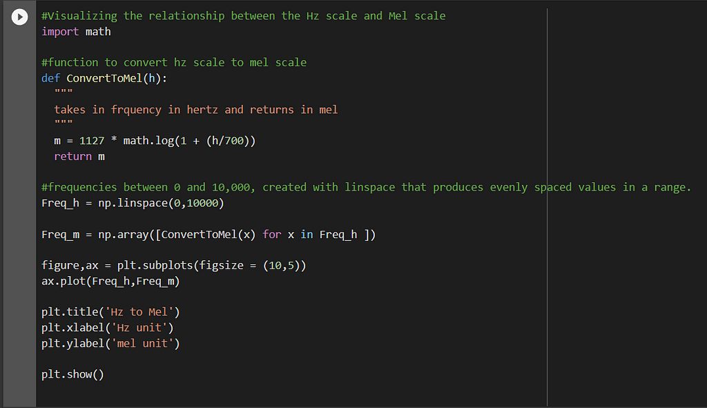
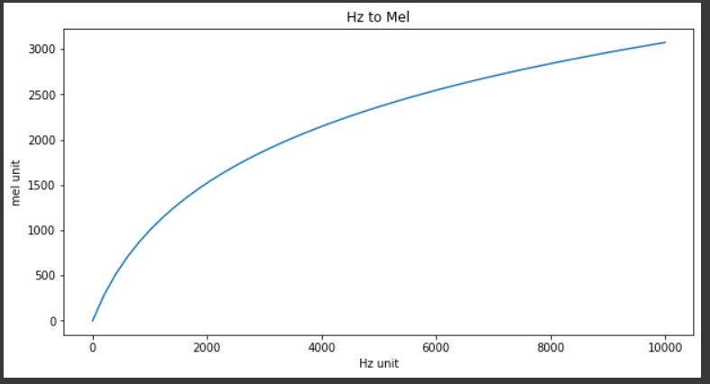
As you can see in the above figure, the distance between frequencies reduces on the mel scale, as the frequency increases, much like the human perception of sound. Lower frequencies have higher gaps in mel, while larger frequencies have a smaller gap, such as between 0 and 2000, and 6000 to 8000.

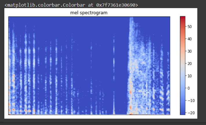
Mel spectrograms are visualized on mel scale as opposed to the frequency scale. This is the fundamental difference.

We also convert our amplitudes to decibels, to get clearer and better outputs.

Db = 20 * log10(amplitude)

The decibel scale is an exponential scale when it comes to the perception of sound. With every increase of 10 decibels, the perception of loudness increases 10 times. Sound at 20 decibels is 10 times louder than at10 decibels. Using mel scale for frequencies and decibel scale for aptitudes, we transform sound closer to human perception, which is key in deep learning. The colors are indicated in the decibel scale and not amplitude.

#create mel spectrograms and conver to decibel scale.

y_spec = librosa.amplitude_to_db(librosa.feature.melspectrogram(y))

#plot mel spectrogram

figure, ax = plt.subplots(figsize=(10,5))

ax.set(title = 'mel spectrogram' )

f= librosa.display.specshow(y_spec,ax=ax)

plt.colorbar(f)

Minimum frequency, maximum frequency, time window length, number of frequency bands, and hop length (number of samples to slide the time window over at each step) become the hyperparameters while creating our spectrograms.

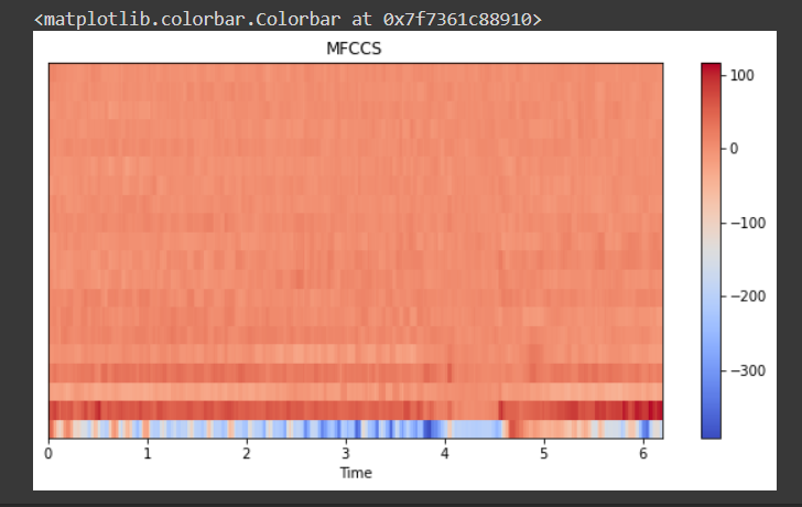
Mel Frequency Cepstral Coefficients (MFCCs) have been popularly used for processing audio signals, especially speech. Thus making it a candidate for a feature in our case study. Discrete cosine transformation is used over the mel spectrogram values to generate MFCCs. The number of coefficients is a hyperparameter and tuned to a problem. MFCCs are successfully applied to voice recognition problems. The Libros library’s default value is 20. The MFCC takes the most important features from the spectrogram that defines the quality of the audio as it is perceived by humans.

#Visualising Mel frequecy cepstral coeffs

#create MFCC

y_mfcc = librosa.feature.mfcc(y)

#plot MFCC

figure, ax = plt.subplots(figsize=(10,5))

ax.set(title = 'MFCCS' )

f= librosa.display.specshow(y_mfcc,ax=ax,x_axis='time')

plt.colorbar(f)

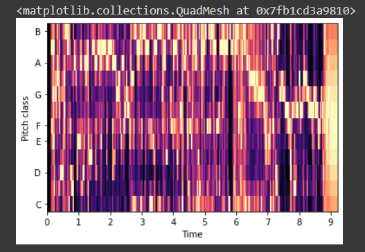
Chromatograms and chroma frequencies:

Pitch is the metric of the elevation of the sound. High sound has a high pitch, low sound has a low pitch. There are seven pitch classes to which each sound belongs.

Chroma filters are used to create chromatograms. The filters project the energy of the recorded sound into 12 bins — the notes and keys. A heat map can be used to visualize the change of pitch over time. By taking a dot product between filters and the Fourier transformed spectrograms, the sounds can be mapped with the set of pitches.

#chroma filter banks

# taking 'sr' and 'n_fft' as 22050 and 4096 respectively

chroma_filter_bank = librosa.filters.chroma(22050 , 4096)

librosa.display.specshow(chroma_filter_bank)

#chroma features of our sound wave

y_chroma = librosa.feature.chroma_stft(y, sr=sr)

librosa.display.specshow(y_chroma, y_axis='chroma', x_axis='time')

Conclusion:

in this part we saw the problem, the data set, and saw the features which would help us build machine learning models on them.

in the next part, we will extract these features and do some EDA on them.

References:

1. High accuracy classification of COVID-19 coughs using Mel-frequency cepstral coefficients and a Convolutional Neural Network with a use case for smart home devices by Dunne et al. Link here
2. Coswara — A Database of Breathing, Cough, and Voice Sounds for COVID-19 Diagnosis by Sharma et al. Link here
3. COVID-19 Artificial Intelligence Diagnosis Using Only Cough Recordings by Laguarta et al. Link here

---

Sound and Acoustic patterns to diagnose COVID [Part 1] was originally published in Towards AI on Medium, where people are continuing the conversation by highlighting and responding to this story.

Join thousands of data leaders on the AI newsletter. It’s free, we don’t spam, and we never share your email address. Keep up to date with the latest work in AI. From research to projects and ideas. If you are building an AI startup, an AI-related product, or a service, we invite you to consider becoming a sponsor.

Published via Towards AI