REGRESSION — HOW, WHY, AND WHEN?

Author(s): Data Science meets Cyber Security

Originally published on Towards AI the World’s Leading AI and Technology News and Media Company. If you are building an AI-related product or service, we invite you to consider becoming an AI sponsor. At Towards AI, we help scale AI and technology startups. Let us help you unleash your technology to the masses.

REGRESSION — HOW, WHY, AND WHEN?

SUPERVISED MACHINE LEARNING — PART 2

REGRESSION:

As we previously saw, the supervised part of machine learning is separated into two categories, and from those two categories, we have already ventured into the realm of classification and the many algorithms employed in the classification process. Regression is the other side of the same coin in which we utilize regression techniques to uncover or establish relationships between the independent factors, features, and dependent variables, as well as the outcome.

The regression procedure allows you to safely decide which elements are most important, which may be overlooked, and how certain factors impact each other.

The ultimate goal is to get many things straightened out so you can be confident in what you want to build or work on finding the solution to your problem.

Simple linear regression is denoted by the formula:

y = β0 + β1 x.

REGRESSION EXAMPLES IN REAL LIFE:

1. Drawing the dots between heavy and reckless driving and the frequent accidents caused in a year.
2. Predicting the sales of a particular product in the company.
3. Medical researchers frequently employ linear regression to examine the association between medicine dose and patients’ blood pressure.
4. Stock forecasts are made by examining historical data on stock prices and trends in order to detect patterns. And much more.

SO EXACTLY, HOW DOES REGRESSION DIFFER FROM CLASSIFICATION?

When we discuss Classification difficulties, we are referring to the categorical values that are important, implying that the output is discrete.

However, in the case of REGRESSION, the situation is reversed; here, the values that matter are numerical, and the output is continuous rather than discrete.

Another significant distinction between the two methods is that, as we saw in the last blog (i.e., world of classification), we used classification techniques to determine decision boundaries and split the entire large dataset into two distinct classes.

However, in Regression, as previously explained, we do not split the dataset into two groups but rather identify the best fit line that can properly predict the outcome.

Finally, another significant distinction between the two techniques is that classification algorithms typically handle issues linked to Natural language processing or computer vision, deep learning such as face detection, speech recognition, picture segmentation, DNA sequence classification, and many more.

When we speak about the regression algorithm, it typically addresses issues linked to elements such as sales, growth, market assessment, consumer demand, and many more such as house price prediction, future stock price prediction, cryptocurrency price prediction, and so on.

We talked a lot about theory let’s get into the practical zone to understand things better:

HOW IS REGRESSION IMPLEMENTED IN ORDER TO SOLVE THE PROBLEMS?

SIMPLE LINEAR REGRESSION:

PROBLEM STATEMENT:

The given data has various attributes of a car, so now we’ll use a linear regression approach to estimate the price of the car with a combination of collected features.

Some of the terminologies to keep in mind while we deal with the practical implementation.

1. PRICE — The cost of the car
2. RELIABILITY — An intermediate measurement for determining the dependability of a vehicle.
3. MILEAGE — The vehicle’s fuel mileage.
4. TYPE — A categorical variable defines the category to which the car belongs.
5. WEIGHT — The weight of the car
6. DISPLACEMENT — Represents the engine displacement of the car
7. HP — Horsepower of the vehicle, a unit that measures its power.

DATA READING:

IMPORTANCE OF DATA READING:

To ensure that the clean and organized data can be utilized to train the model further and avoid any misunderstanding when working with large datasets, it is necessary to pre-process and begin the cleaning of the data, i.e., transforming raw data into clean data.
Reading data is crucial to developing the model and moving ahead.

getwd()

## Load the data
cars_data  <- read.csv(file = "cars.csv")

DATA UNDERSTANDING:

In this phase, we‘ll check the number of observations and attributes taking place. Classify the independent and dependent variables.

NOTE: In linear regression, the dependent variable is a continuous variable.

Here, we’ll predict the dependent variable with one independent variable.

EXAMPLE: We will consider the PRICE as the dependent variable and the DISPLACEMENT of the car as the independent variable.

dim(cars_data)

str(cars_data)

head(cars_data)

tail(cars_data)

summary(cars_data)

DATA TYPE CONVERSION:

Attribute values can be implicitly or explicitly transformed. The user is not aware of implicit conversions. SQL Server translates data from one data type to another instantly. When comparing a small-int to an int, for instance, the small-int is implicitly transformed into an int before the comparison is performed.

#Convert "Reliability" to factor variable
cars_data[, "Reliability"] <- as.factor(as.character(cars_data[, "Reliability"]))

cars_data[, "Country"] <- as.factor(as.character(cars_data[, "Country"]))
cars_data[, "Type"] <- as.factor(as.character(cars_data[, "Type"]))

str(cars_data)

HANDLING VALUES:

So that we don’t have any null/blank spaces creating havoc in our model.

## Look for Missing Values
sum(is.na(cars_data))

colSums(is.na(cars_data))

#Install the DMwR2 package incase you haven't.
install.packages("DMwR2", dependencies=TRUE)

## Imputing missing values
library(DMwR2)
cars_data=centralImputation(cars_data)

sum(is.na(cars_data))

sum(is.na(cars_data))

DATA EXPLORATORY ANALYSIS:

Exploratory Data Analysis is the crucial process of doing preliminary investigations on data in order to good detection rate, identify irregularities, test hypotheses, and validate assumptions using statistical results and visualizations.

#Plot the Dependent and  Independent variables
# _*Scatter Plot*_ helps to view the relationship between two continuous variables
 
options(repr.plot.width = 10, repr.plot.height = 10)
par(mfrow = c(2,2)) # Splits the plotting pane 2*2
 
plot(cars_data$Weight, cars_data$Price, xlab = "Weight",
    ylab = "Price", main = "Weight vs Price")
 
plot(cars_data$Mileage, cars_data$Price, xlab = "Mileage",
    ylab = "Price", main = "Mileage vs Price")
 
plot(cars_data$Disp., cars_data$Price, xlab = "Displacement",
    ylab = "Price", main = "Displacement vs Price")
 
plot(cars_data$HP, cars_data$Price, xlab = "Horse Power",
    ylab = "Price", main = "Horse Power vs Price")

SPLITTING THE DATA INTO TRAINING AND VALIDATION SETS:

The major goal of dividing the dataset into a validation set is to avoid our models from overfitting, which occurs when the algorithm is very effective at categorizing items in the test dataset but struggles to generalize the practices and knowledge predictions on data it has not encountered before.

1:100

sample(1:100,size=10)

cars_data[c(1,10),]

## Split row numbers into 2 sets
set.seed(1)
train_rows = sample(1:nrow(cars_data), size=0.7*nrow(cars_data))
validation_rows = setdiff(1:nrow(cars_data),train_rows)

train_rows

validation_rows

## Subset into Train and Validation sets
train_data <- cars_data[train_rows,]
validation_data <- cars_data[validation_rows,]

## View the dimensions of the data
dim(cars_data)
dim(train_data)
dim(validation_data)

LET’S BUILD A MODEL NOW:

names(train_data)

# lm function is used to fit linear models
LinReg = lm(Price ~ Disp., data = train_data)

## Summary of the linear model
summary(LinReg)

GITHUB GIST ❤️

In case you wanna run the code and interpret the results:

2. MULTIPLE LINEAR REGRESSION:

As we have seen in the simple linear regression, the computation in simple linear regression is to calculate the distance between a dependent variable ‘Y’ and an independent variable ‘X’.

When we talk about Multiple linear regression, the concept is almost the same, or we can say that it is an augmentation of simple linear regression where instead of finding the relationship between dependent and independent variables, we find the relationship between the dependent variable ‘Y’ and explanatory variable ‘P.’

Multiple linear regression is denoted by the formula:

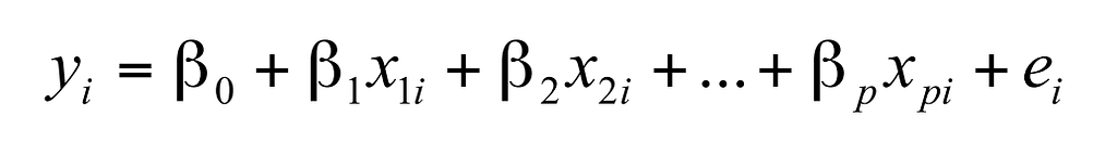
NOTATIONS:

β0 = Constant term

β1 and βP = Explanatory variable

INTERESTING TIDBIT:

We use the term ‘LINEAR’ in Multiple linear regression because we always believe that the ‘Y’ is directly connected to the linear combination of the explanatory variable ‘P’ when we utilize regression.

REAL-LIFE EXAMPLES WHERE WE USE MULTIPLE LINEAR REGRESSION:

1. Attempting to forecast a person’s earnings based on a variety of sociodemographic variables.
2. Attempting to forecast total assessment success of ‘A’ level students based on the values of a collection of examination results at the range of 16.
3. Attempting to calculate systolic or diastolic blood pressure based on social and economical, and lifestyle factors (employment, drinking, smoking, age, etc.).

LET’S SEE THE PRACTICAL IMPLEMENTATION OF SOME CASE STUDIES TO GET THINGS MORE CLEAR:

3. LOGISTIC REGRESSION:

Logistic regression is a statistical analytic approach that uses pre—existing data of an original dataset to estimate a binary result, such as yes or no. A logistic regression model forecasts a dependent variable by examining the connection between one or more existing independent variables.

We have previously seen a lot about logistic regression in the classification blog; if you want to perform a fast refresher, turn to the first technique of types of classification algorithm to learn more about it.

In terms of logistic regression types, there are three primary subtypes in LOGISTIC REGRESSION:

1. BINARY LOGISTIC REGRESSION:

When we think about binary logistic regression, the first and only thing that springs to mind is 0 and 1 (binary numbers), and that is exactly what it is. The response has two possible outcomes: 0 or 1.

This is the most common of the three approaches.

2. MULTINOMIAL LOGISTIC REGRESSION:

When using the multinomial logistic regression technique, the variable of interest can have more than three outcomes, and the order is not fixed, and as previously established, the outcome does not have to be a binary integer.

EXAMPLE: If Netflix wishes to categorize the top ten most viewed trending shows of the month of November, logistic regression will assist Netflix in determining the viewing time of each show in a certain area or nation. Then Netflix may begin the marketing by advertising the top ten series with the most watching hours.

3. ORDINAL LOGISTIC REGRESSION:

The final technique is ordinal logistic regression, in which the model contains a dependent variable with three or more possibilities, but unlike multinomial logistic regression, where the order is not specified, the values in ordinal logistic regression have a definite order.

EXAMPLE: Universities assign grades based on marks ranging from A to D.

IMPLEMENTATION IN PRACTICE BY UNDERSTANDING THE CASE STUDY:

HAD FUN LEARNING REGRESSION? BECAUSE WE HAD FUN WRITING FOR YOU GUYS!

FOLLOW US FOR THE SAME FUN TO LEARN DATA SCIENCE BLOGS AND ARTICLES: 💙

LINKEDIN: https://www.linkedin.com/company/dsmcs/

INSTAGRAM: https://www.instagram.com/datasciencemeetscybersecurity/?hl=en

GITHUB: https://github.com/Vidhi1290

TWITTER: https://twitter.com/VidhiWaghela

MEDIUM: https://medium.com/@datasciencemeetscybersecurity-

WEBSITE: https://www.datasciencemeetscybersecurity.com/

— Team Data Science meets Cyber Security ❤️💙

---

REGRESSION — HOW, WHY, AND WHEN? was originally published in Towards AI on Medium, where people are continuing the conversation by highlighting and responding to this story.

Join thousands of data leaders on the AI newsletter. It’s free, we don’t spam, and we never share your email address. Keep up to date with the latest work in AI. From research to projects and ideas. If you are building an AI startup, an AI-related product, or a service, we invite you to consider becoming a sponsor.

Published via Towards AI