Proving the Convexity of Log-Loss for Logistic Regression

Author(s): Towards AI Editorial Team

Originally published on Towards AI.

Unpacking Log Loss Error Function’s Impact on Logistic Regression

Photo by DeepMind on Unsplash

Author(s): Pratik Shukla

“Courage is like a muscle. We strengthen it by use.” — Ruth Gordo

Table of Contents:

1. Proof of convexity of the log-loss function for logistic regression
2. A visual look at BCE for logistic regression
3. Resources and references

Introduction

In this tutorial, we will see why the log-loss function works better in logistic regression. Here, our goal is to prove that the log-loss function is a convex function for logistic regression. Once we prove that the log-loss function is convex for logistic regression, we can establish that it’s a better choice for the loss function.

Logistic regression is a widely used statistical technique for modeling binary classification problems. In this method, the log-odds of the outcome variable is modeled as a linear combination of the predictor variables. To estimate the parameters of the model, the maximum likelihood method is used, which involves optimizing the log-likelihood function. The log-likelihood function for logistic regression is typically expressed as the negative sum of the log-likelihoods of each observation. This function is known as the log-loss function or binary cross-entropy loss. In this blog post, we will explore the convexity of the log-loss function and why it is an essential property in optimization algorithms used in logistic regression. We will also provide a proof of the convexity of the log-loss function.

Proof of convexity of the log-loss function for logistic regression:

Let’s mathematically prove that the log-loss function for logistic regression is convex.

We saw in the previous tutorial that a function is said to be a convex function if its second derivative is >0. So, here we’ll take the log-loss function and find its second derivative to see whether it’s >0 or not. If it’s >0, then we can say that it is a convex function.

Here we are going to consider the case of a single trial to simplify the calculations.

Step — 1:

The following is a mathematical definition of the binary cross-entropy loss function (for a single trial).

Figure — 1: Binary Cross-Entropy loss for a single trial

Step — 2:

The following is the predicted value (ŷ) for logistic regression.

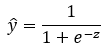Figure — 2: The predicted probability for the given example

Step — 3:

In the following image, z represents the linear transformation.

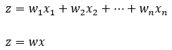Figure — 3: Linear transformation in forward propagation

Step — 4:

After that, we are modifying Step — 1 to reflect the values of Step — 3 and Step — 2.

Figure — 4: Binary Cross-Entropy loss for logistic regression for a single trial

Step — 5:

Next, we are simplifying the terms in Step — 4.

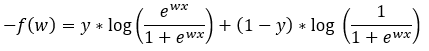Figure — 5: Binary Cross-Entropy loss for logistic regression for a single trial

Step — 6:

Next, we are further simplifying the terms in Step — 5.

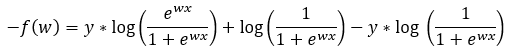Figure — 6: Binary Cross-Entropy loss for logistic regression for a single trial

Step — 7:

The following is the quotient rule for logarithms.

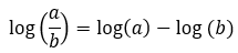Figure — 7: The quotient rule for logarithms

Step — 8:

Next, we are using the equation from Step — 7 to further simplify Step — 6.

Figure — 8: Binary Cross-Entropy loss for logistic regression for a single trial

Step — 9:

In Step — 8, the value of log(1) is going to be 0.

Figure — 9: The value of log(1)=0

Step — 10:

Next, we are rewriting Step — 8 with the remaining terms.

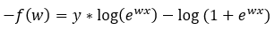Figure — 10: Binary Cross-Entropy loss for logistic regression for a single trial

Step — 11:

The following is the power rule for logarithms.

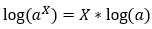Figure — 11: Power rule for logarithms

Step — 12:

Next, we will use the power rule of logarithms to simplify the equation in Step — 10.

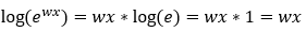Figure — 12: Applying the power rule

Step — 13:

Next, we are replacing the values in Step — 10 with the values in Step — 12.

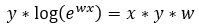Figure — 13: Using the power rule for logarithms

Step — 14:

Next, we are substituting the value of Step — 13 into Step — 10.

Figure — 14: Binary Cross-Entropy loss for logistic regression for a single trial

Step — 15:

Next, we are multiplying Step — 14 by (-1) on both sides.

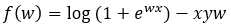Figure — 15: Binary Cross-Entropy loss for logistic regression for a single trial

Finding the First Derivative:

Step — 16:

Next, we are going to find the first derivative of f(x).

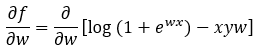Figure — 16: Finding the first derivative of f(w)

Step — 17:

Here we are distributing the partial differentiation sign to each term.

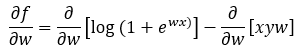Figure — 17: Finding the first derivative of f(w)

Step — 18:

Here we are applying the derivative rules.

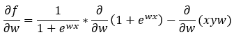Figure — 18: Finding the first derivative of f(w)

Step — 19:

Here we are finding the partial derivative of the last term of Step — 18.

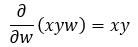Figure — 19: Finding the first derivative of f(w)

Step — 20:

Here we are finding the partial derivative of the first term of Step — 18.

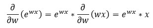Figure — 20: Finding the first derivative of f(w)

Step — 21:

Here we are putting together the results of Step — 19 and Step — 20.

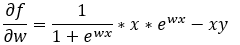Figure — 21: Finding the first derivative of f(w)

Step — 22:

Next, we are rearranging the terms of the equation in Step — 21.

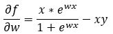Figure — 22: Finding the first derivative of f(w)

Step — 23:

Next, we are rewriting the equation in Step — 22.

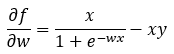Figure — 23: Finding the first derivative of f(w)

Finding the Second Derivative:

Step — 24:

Next, we are going to find the second derivative of the function f(x).

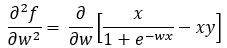Figure — 24: Finding the second derivative of f(w)

Step — 25:

Here we are distributing the partial derivative to each term.

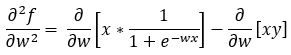Figure — 25: Finding the second derivative of f(w)

Step — 26:

Next, we are simplifying the equation in Step — 25 to remove redundant terms.

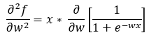Figure — 26: Finding the second derivative of f(w)

Step — 27:

Here is the derivative rule for 1/f(x).

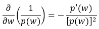Figure — 27: The derivative rule for 1/f(x)

Step — 28:

Next, we are finding the relevant term to plug-in in Step — 27.

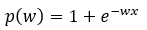Figure — 28: Value of p(w) for derivative of 1/p(w)

Step — 29:

Here we are finding the partial derivative term for Step — 27.

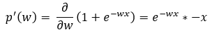Figure — 29: Value of p’(w) for derivative of 1/p(w)

Step — 30:

Here we are finding the squared term for Step — 27.

Figure — 30: Value of p(w)² for derivative of 1/p(w)

Step — 31:

Here we are putting together all the terms of Step — 27.

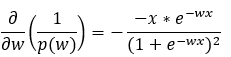Figure — 31: Calculating the value of the derivative of 1/p(w)

Step — 32:

Here we are simplifying the equation in Step — 31.

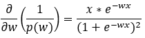Figure — 32: Calculating the value of the derivative of 1/p(w)

Step — 33:

Next, we are putting together all the values in Step — 26.

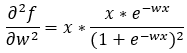Figure — 33: Finding the second derivative of f(w)

Step — 34:

Next, we are further simplifying the terms in Step — 33.

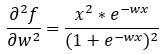Figure — 34: Finding the second derivative of f(w)

Alright! So, now we have the second derivative of the function f(x). Next, we need to find out whether this will be >0 for all the values of x or not. If it is >0 for all the values of x, then we can say that the binary cross-entropy loss is convex for logistic regression.

As we can see that the following terms from Step — 34 are always going to be ≥0 because the square of any number is always ≥0.

Figure — 35: The square of any term is always ≥0 for any value of x

Now, we need to determine whether or not the value of e^(-wx) is >0. To do that, let’s first find the range of the function e^(-wx) in the domain [-∞,+∞]. To further simplify the calculations, we will consider the function e^-x instead of e^-wx. Please note that scaling a function does not change the range of the function if the domain is [-∞,+∞]. Let’s first plot the graph of e^-x to understand its range.

Figure — 36: Graph of e^-x for the domain of [-10, 10]

From the above graph we can derive the following conclusion:

1. As the value of x moves towards negative infinity (-∞), the value of e^-x moves towards infinity (+∞).

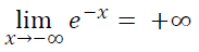Figure — 37: The value of e^-x as x approaches -∞

2. As the value of x moves towards 0, the value of e^-x moves towards 1.

Figure — 38: The value of e^-x as x approaches 0

3. As the value of x moves towards positive infinity (+∞), the value of e^-x moves towards 0.

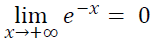Figure — 40: The value of e^-x as x approaches +∞

So, we can say that the range of the function f(x)=e^-x is [0,+∞]. Based on the calculations, we can say that the function f(x)=e^-wx is always going to be ≥0.

Alright! So, we have concluded that all the terms of the equation in Step — 34 are≥0. Hence, we can say that the function f(x) is a convex function for logistic regression.

Important Note:

If the value of the second derivative of the function is 0, then there is a possibility that the function is neither concave nor convex. But, let’s not worry too much about it!

A Visual Look at BCE for Logistic Regression:

The binary cross entropy function for logistic regression is given by…

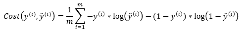Figure — 41: Binary Cross Entropy Loss

Now, we know that this is a binary classification problem. So, there can be only two possible values for Yi (0 or 1).

Step — 1:

The value of cost function when Yi=0.

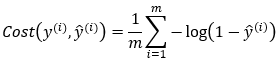Figure — 42: Binary Cross Entropy Loss when Y=0

Step — 2:

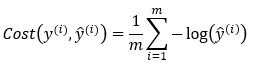Figure — 43: Binary Cross Entropy Loss when Y=1

Now, let’s consider only one training example.

Step — 3:

Now, let’s say we have only one training example. It means that n=1. So, the value of the cost function when Y=0,

Figure — 44: Binary Cross Entropy Loss for a single training example when Y=0

Step — 4:

Now, let’s say we have only one training example. It means that n=1. So, the value of the cost function when Y=1,

Figure — 45: Binary Cross Entropy Loss for a single training example when Y=1

Step — 5:

Now, let’s plot the function graph in Step — 3.

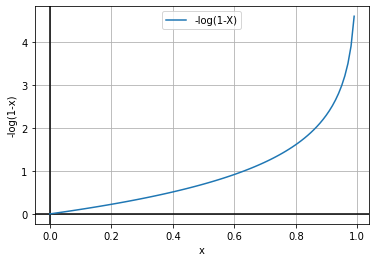Figure — 46: Graph of -log(1-X)

Step — 6:

Now, let’s plot the function graph in Step — 4.

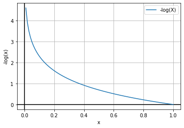Figure — 47: Graph of -log(X)

Step — 7:

Let’s put the graphs in Step — 5 and Step — 6 together.

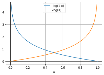Figure — 48: Graph of -log(1-X) and -log(X)

The above graphs follow the definition of the convex function (“A function of a single variable is called a convex function if no line segments joining two points on the graph lie below the graph at any point”). So, we can say that the function is convex.

Conclusion:

In conclusion, we have explored the concept of convexity and its importance in optimization algorithms used in logistic regression. We have demonstrated that the log-loss function is convex, which implies that its optimization problem has a unique global minimum. This property is crucial for ensuring the stability and convergence of optimization algorithms used in logistic regression. By proving the convexity of the log-loss function, we have shown that the optimization problem in logistic regression is well-posed and can be efficiently solved using standard convex optimization methods. Moreover, our proof provides a deeper understanding of the mathematical foundations of logistic regression and lays the groundwork for further research and development in this field.

Buy Pratik a Coffee!

Citation:

For attribution in academic contexts, please cite this work as:

Shukla, et al., “Proving the Convexity of Log Loss for Logistic Regression”, Towards AI, 2023

BibTex Citation:

@article{pratik_2023, 
 title={Proving the Convexity of Log Loss for Logistic Regression}, 
 url={https://pub.towardsai.net/proving-the-convexity-of-log-loss-for-logistic-regression-49161798d0f3}, 
 journal={Towards AI}, 
 publisher={Towards AI Co.}, 
 author={Pratik, Shukla},
 editor={Binal, Dave}, 
 year={2023}, 
 month={Feb}
}

---

Proving the Convexity of Log-Loss for Logistic Regression was originally published in Towards AI on Medium, where people are continuing the conversation by highlighting and responding to this story.

Join thousands of data leaders on the AI newsletter. Join over 80,000 subscribers and keep up to date with the latest developments in AI. From research to projects and ideas. If you are building an AI startup, an AI-related product, or a service, we invite you to consider becoming a sponsor.

Published via Towards AI