Predicting Genres from Movie Dialogue

Last Updated on May 18, 2021 by Editorial Team

Author(s): Harry Roper

Natural Language Processing

Multi-label NLP Classification

“Some day, and that day may never come, I will call upon you to do a service for me. But until that day, consider this justice a gift on my daughter’s wedding day.” — Don Vito Corleone, The Godfather (Francis Ford Coppola, 1972)

Anyone with even a mild interest in cinema would likely be able to identify the movie that spawned the above line, not least infer its genre. Such is the power of a good quote.

But does the majesty of cinematic dialogue also resonate in the ears of a machine? This article aims to employ the features of Natural Language Processing (NLP) to build a classification model to predict movies’ genres based on exchanges from their dialogue.

The model produced will be an example of a multi-label classifier, in that each instance in the data set can be assigned a positive class for zero or more labels simultaneously. Note that this differs from a multi-class classifier, since the vector of possible classes is still binary.

Predicting movie genres based on synopses is a relatively common example within the area of multi-label NLP models. There appears, however, to be little to no work using movie dialogue as input. The motivation behind this post was hence to explore whether text patterns could be uncovered in movies’ dialogue to act as indicators of their genres.

The process of construction will fall under three main stages:

1. Compiling, cleaning, and preprocessing the training data set
2. Exploratory analysis of the training data
3. Building and evaluating the classification model

Part I: Compiling the Training Data Set

The data for this project was obtained via a publication from Cornell University (credited in the acknowledgements section).

Of the files provided, there are three data sets of interest to the project:

• Movie Conversations: exchanges of dialogue listed as combinations of line IDs along with the corresponding movie IDs
• Movie Lines: the text of each line of dialogue along with its corresponding line ID
• Movie Titles Metadata: attributes of the movies included in the data, such as titles and genres

To compile a classified set of training data from the raw files, we will need to extract the necessary data, transform it into a workable format, and load it into a database which we can later read in.

Extracting, Transforming, and Loading the Training Data

The ETL pipeline used to produce the final training set will comprise the following steps:

1. Reading the data from each of the three text files into pandas dataframes
2. Assigning a conversation ID to each exchange contained in the conversations data set
3. Melting the conversations dataframe such that each line of dialogue appears on a separate row with the corresponding conversation ID
4. Joining the melted dataframe with the lines data set to retrieve the actual text for each line ID
5. Joining the separate rows via the conversation ID such that the entirety of each exchange appears in text format on an individual row
6. Finally, joining the dataframe of text conversations with the movie metadata to retrieve the genres for each text document, and loading the final dataframe to a SQLite database

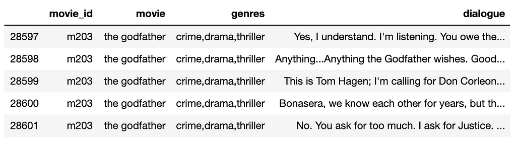
Once the ETL pipeline has been run on the raw files, the training data set will appear like so:

Reformatting the Target Variable

Thinking ahead to the modelling stage, we need to reformat the genres column into a target variable suitable to be fed into a machine learning algorithm.

The labels in the genres column are listed as strings separated by commas, so to create the target variable we can use a variation of one-hot encoding. This involves creating a separate column in the dataframe for each unique genre label to indicate whether the label is contained within the main genres column, with 1 for yes and 0 for no.

genres = df['genres'].tolist()
genres = ','.join(genres)
genres = genres.split(',')
genres = sorted(list(set(genres)))
for genre in genres:
    df[genre] = df['genres'].apply(lambda x: 1 if genre in x else 0)

The set of binary genre columns will as a target variable matrix in which each movie can be assigned any number of 24 unique labels.

Part II: Exploratory Analysis of the Training Data

Now that we’ve reworked the data into a suitable format, let’s begin some exploration to draw some insights before we construct the model. We can start by taking a look at the number of individual genre labels to which each movie is assigned:

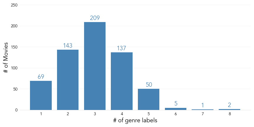
Most movies in our data set are assigned 2–4 genre labels. When we consider that there are 24 possible labels in total, this highlights that we can expect our target variable matrix to contain far more negative classifications than positive.

This provides a valuable insight to take into the modelling stage, in that we can observe a significant class imbalance in the training data. To assess this imbalance numerically:

df[genres].mean().mean()
>>> 0.12317299038986919

The above indicates that only 12% of the data set’s labels belong to the positive class. This factor should be given particular attention when deciding upon a method of evaluating the model.

Let’s also assess the number of positive instances we have for each genre label:

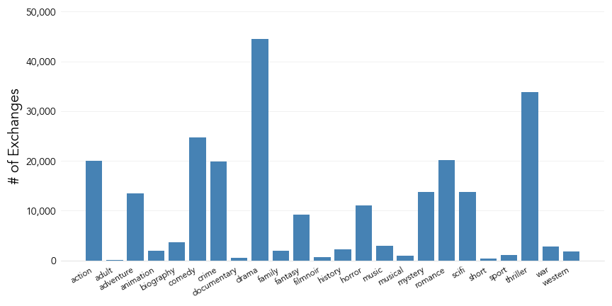
On top of the class imbalance identified previously, the chart above uncovers that the data also has a significant label imbalance, in that some genres (such as Drama) have many more positive instances on which to train the model than others (such as Film noir).

This is likely to have implications on the model’s success between different genres.

Discussing the Results of the Analysis

The analysis above uncovers two key insights about our training data:

1. The class distribution is heavily imbalanced in favour of the negative.

In the context of this model, class imbalance is difficult to amend. A typical method for correcting class imbalance is synthetic oversampling: the creation of new instances of the minority class with feature values close to those of the genuine instances.

However, this method is generally unsuitable for a multi-label classification problem, since any credible synthetic instances would display the same issue. The class imbalance therefore reflects the reality of the situation, in that a movie is only assigned a small number of all possible genres.

We should keep this in mind when choosing the performance metric(s) with which to evaluate the model. If, for example, we judge the model based on accuracy (correct classifications as a proportion of total classifications), we could expect to achieve a score of c.88% simply by predicting every instance as a negative (considering that only 12% of training labels are positive).

Metrics such as precision (the proportion of actual positives that were classified correctly) and recall (the proportion of positive classifications made that were correct) are more suitable in this context.

2. The distribution of positive classes is imbalanced amongst labels.

If we’re to use the current data set to train the model, we must accept the fact that the model will likely be able to classify some genres more accurately than others, simply because of the increased availability of data.

The most effective way of dealing with this issue would probably to return to the data set compiling stage and search for additional sources of training data with which to amend the label imbalances. This is something that could be considered when working on an improved version of the model.

Part III: Building the Classification Model

Natural Language Processing (NLP)

At present, the data for our model’s features is still in the raw text format in which it was provided. To transform the data into a format suitable for machine learning, we’ll need to employ some NLP techniques.

The steps involved to turn a corpus of text documents into a numerical feature matrix will be as follows:

1. Clean the text to remove all punctuation and special characters
2. Separate the individual words in each document into tokens
3. Lemmatise the text (grouping inflected words together, such as replacing the words “learning” and “learnt” with “learn”)
4. Remove whitespace from tokens and set them to lower case
5. Remove all stop words (e.g. “the”, “and”, “of” etc)
6. Vectorise each document into word counts
7. Perform a term frequency-inverse document frequency (TF-IDF) transformation on each document to smoothen counts based on the frequency of terms within the corpus

We can write the text cleaning operations (steps 1–5) into a single function:

def tokenize(text):
    text = re.sub('[^a-zA-Z0-9]', ' ', text)
    tokens = word_tokenize(text)
    lemmatizer = WordNetLemmatizer()
    clean_tokens = (lemmatizer.lemmatize(token).lower().strip() for token in tokens if token \
                    not in stopwords.words('english'))
    return clean_tokens

that can then be passed as the tokeniser into scikit-learn’s CountVectorizer function (step 6), and finish the process with the TfidfTransformer function (step 7).

Implementing a Machine Learning Pipeline

The feature variables need to undergo the NLP transformation before they can be passed into a classification algorithm. If we were to run the transformation on the entirety of the data set, it would technically cause data leakage, since the count vectorisation and TF-IDF transformation would be based on data from both the training and testing sets.

To combat this, we could split the data first and then run the transformations. However, this would mean completing the process once for the training data, again for the testing data, and a third time for any unseen data we wanted to classify, which would be somewhat cumbersome.

The most effective way to circumvent this issue is to include both the NLP transformations and classifier as steps in a single pipeline. With a decision tree classifier as the estimator, the pipeline for an initial baseline model would be as follows:

pipeline = Pipeline([
    ('vect', CountVectorizer(tokenizer=tokenize)),
    ('tfidf', TfidfTransformer()),
    ('clf', MultiOutputClassifier(DecisionTreeClassifier()))
    ])

Note that we need to specify the estimator as a MultiOutputClassifier. This is to indicate that the model should return a prediction for each of the specified genre labels for each instance.

Evaluating the Baseline Model

As discussed previously, the class imbalance in the training data needs to be considered when evaluating the performance of the model. To illustrate this point, let’s take a peek at the accuracy of the baseline model.

As well as making considerations for class imbalance, we also need to adjust some of the evaluation metrics to cater for multi-label output since, unlike in single label classification, each predicted instance is no longer a hard right or wrong. For example, an instance for which the model classifies 20 of the 24 possible labels correctly should be considered more of a success than an instance for which none of the labels are classified correctly.

For readers interested in diving deeper into evaluation methods of multi-label classification models, I can recommend A Unified View of Multi-Label Performance Measures (Wu & Zhou, 2017).

One accepted measure of accuracy in multi-label classification is Hamming loss: the fraction of the total number of predicted labels that are misclassified. Subtracting the Hamming loss from one gives us an accuracy score:

1 - hamming_loss(y_test, y_pred)
>>> 0.8667440038568157

An 86.7% accuracy score initially seems like a great result. However, before we pack up and consider the project a success, we need to consider that the class imbalance discussed previously likely means that this score is overly generous.

Let’s compare the Hamming loss to the model’s precision and recall. To return the average scores across labels weighted on each label’s number of positive classes, we can pass average=’weighted’ as an argument into the functions:

precision_score(y_test, y_pred, average='weighted')
>>> 0.44485346325188513
recall_score(y_test, y_pred, average='weighted')
>>> 0.39102002566871064

The far more conservative results for precision and recall likely paint a truer picture of the model’s capabilities, and indicate that the generosity of the accuracy measure was due to the abundance of true negatives.

With this in mind, we’ll use the F1 score (the harmonic mean between precision and recall) as the principal metric when evaluating the model:

f1_score(y_test, y_pred, average='weighted')
>>> 0.41478130331069335

Comparing Performance Across Labels

When exploring the training data, we hypothesised that the model would perform more effectively for some genres than others due to the imbalance in the distribution of positive classes across labels. Let’s ascertain whether this is the case by finding the F1 score for each genre label and plotting it against the total number of training documents for that genre.

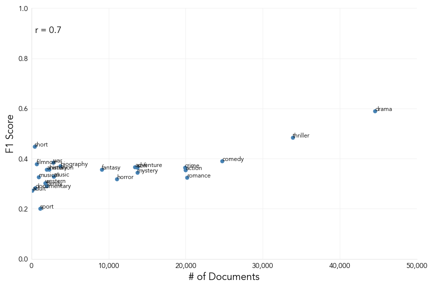
Here we can observe a relatively strong positive correlation (a Pearson’s coefficient of 0.7) between a label’s F1 score and its total number of training documents, confirming our suspicions.

As mentioned previously, the best way around this would be to collect a more balanced data set when building a second version of the model.

Improving the Model: Selecting a Classification Algorithm

Let’s test out some other classification algorithms to see which produces the best results on the training data. To do this, we can loop through a list of the models equipped to deal with multi-label classification and print the weighted average F1 score for each one.

Before running the loop, let’s add an additional step to the pipeline: singular value decomposition (TruncatedSVD). This is a form of dimensionality reduction, which identifies the most meaningful properties of the feature matrix and removes what’s left over. It’s similar to principal component analysis (PCA), but can be used on sparse matrices.

I actually found that adding this step slightly hampered the model’s score. However, it vastly reduced the computational runtime, so I’d consider it a worthwhile trade-off.

We should also switch from evaluating the model over a single training and testing split to using the average score from a cross validation, since this will give a more robust measure of performance.

tree = DecisionTreeClassifier()
forest = RandomForestClassifier()
knn = KNeighborsClassifier()

models = [tree, forest, knn]
model_names = ['tree', 'forest', 'knn']

for model in models:
    pipeline = Pipeline([
    ('vect', CountVectorizer(tokenizer=tokenize)),
    ('tfidf', TfidfTransformer()),
    ('svd', TruncatedSVD()),
    ('clf', MultiOutputClassifier(model))
    ])
    cv_scores = cross_val_score(pipeline, X, y, scoring='f1_weighted', cv=4, n_jobs=-1)
    score = round(np.mean(cv_scores), 4)
    scores.append(score)

model_compare = pd.DataFrame({'model': model_names, 'score': scores})

print(model_compare)
>>> model   score
>>> 0    tree  0.2930
>>> 1  forest  0.2274
>>> 2     knn  0.2284

Rather surprisingly, the decision tree used in the baseline model actually produced the best score of all the models tested. We’ll keep this as our estimator as we move onto the hyper-parameter tuning.

Improving the Model: Tuning Hyper-Parameters

As a final step in building the best model, we can run a cross validation grid search to find the most effective values for the parameters.

Since we’re using a pipeline to fit the model, we can define parameter values to test not only for the estimator, but also the NLP stages, such as the vectoriser.

pipeline = Pipeline([
    ('vect', CountVectorizer(tokenizer=tokenize)),
    ('tfidf', TfidfTransformer()),
    ('svd', TruncatedSVD()),
    ('clf', MultiOutputClassifier(DecisionTreeClassifier()))
    ])

parameters = {
    'vect__ngram_range': [(1, 1), (1, 2)],
    'clf__estimator__max_depth': [250, 500, 1000],
    'clf__estimator__min_samples_split': [1, 2, 6]
}

cv = GridSearchCV(pipeline, param_grid=parameters, scoring='f1_weighted', cv=4, n_jobs=-1, verbose=10)
cv.fit(X, y)

Once the grid search is complete, we can view the parameters and score for our final, tuned model:

print(cv.best_params_)
>>> {'clf__estimator__max_depth': 500, 'clf__estimator__min_samples_split': 2, 'vect__ngram_range': (1, 1)}
print(cv.best_score_)
>>> 0.29404722954784424

The hyper-parameter tuning has allowed us to very marginally improve the model’s performance by .1 of a percentage point, giving a final F1 score of 29.4%. This means that we can expect the model to classify just under a third of the true positives correctly.

Closing Remarks

In summary, we were able to build a model that attempts to predict a movie’s genres from its dialogue by:

1. Manipulating the text corpus obtained from the Cornell University publication to create a training data set
2. Employing NLP techniques to transform the text data into a matrix of feature variables
3. Building a baseline classifier using a machine learning pipeline, and improving the model by evaluating performance metrics suitable in a multi-label classification context with a significant class imbalance

The final model can be used to generate predictions for new dialogue exchanges. The following example uses a quote from Carnival of Souls (Herk Harvey, 1962):

def predict_genres(text):
    pred = pd.DataFrame(cv.predict([text]), columns=genres)
    pred = pred.transpose().reset_index()
    pred.columns = ['genre', 'prediction']
    predictions = pred[pred['prediction']==1]['genre'].tolist()
    return predictions

line = "It's funny... the world is so different in the daylight. In the dark, your fantasies get so out of hand. \
But in the daylight everything falls back into place again."

print(predict_genres(line))
>>> ['family', 'scifi', 'thriller']

So what’s the final verdict? Can we propose to IMDb to adopt our model as a means of automating their genre categorisation? At this stage, probably not. However, the model created in this post should be a good enough starting point, with opportunities for making improvements in future versions by, for example, compiling a larger data set that’s more balanced across the different genres.

Readers interested in downloading the data set, running the ETL pipeline, or checking out the code written to build the model can do so in this repository of my Github. Feedback, questions, and suggestions on improving the model are always welcome.

Acknowledgements

Cristian Danescu-Niculescu-Mizil. Cornell Movie — Dialogs Corpus. Cornell University 2011

Xi-Zhu Wu and Zhi-Hua Zhou. A Unified View of Multi-Label Performance Measures. ICML 2017

---

Predicting Genres from Movie Dialogue was originally published in Towards AI on Medium, where people are continuing the conversation by highlighting and responding to this story.

Published via Towards AI