Outline a Smaller Class With the Custom Loss Function

Author(s): Konstantin Pluzhnikov

Originally published on Towards AI the World’s Leading AI and Technology News and Media Company. If you are building an AI-related product or service, we invite you to consider becoming an AI sponsor. At Towards AI, we help scale AI and technology startups. Let us help you unleash your technology to the masses.

A short guide to you for taking the most from classification when dealing with imbalanced datasets

Why use a custom loss function?

There may be situations when the accuracy metric is insufficient to get the expected results. We may want to reduce the false negative (FN) or false positive (FP) rate. It may be beneficial when a dataset is imbalanced and the result we seek belongs to a smaller class.

Where to apply

1. Fraud detection. We want to reduce false negative samples (e.g., a model treats a transaction as usual when it is doubtful). A goal is to minimize the risk of fraudulent transactions bypassing unnoticed (even if the false positive rate would grow).

2. Disease identification. It has the same logic. We want to increase the chances of catching the disease, even if we get more FP cases to sort out in the future.

3. Pick an outsider in a sports match. Let’s assume a game with two outcomes (win/loss of a favorite). But we want to find out if an outsider has a chance. A balanced model will perform “cherry picking” most of the time because it is an easy way to predict a favorite’s win. The way out is to penalize false negatives (cases when a model predicts the victory of a stronger team, but the accurate label is a loss of a favorite).

We do not want high FP rates in the first two cases because it would increase resource usage to confirm that sample is not a fraud/disease. So model optimization remains necessary.

The bridge between original and custom logloss

An ordinary gradient boosting algorithm (the algorithm) makes the following steps. It gets the predicted value (let’s call it “predt”, in the form of logit or logitraw depending on the library we use) and a respective true label (let’s call it “y”), then it estimates the value of the logloss function. It performs these actions line by line to calculate the cumulative loss function value.

The logloss has the following formula:

where N— number of samples, y— true label, log — natural logarithm.

p_i — the probability of the ith sample being 1(sigmoid function):

where m is the number of features, zis linear regression where ware weights of features, xare feature values.

The next step is to update the features’ weights to minimize the loss. The algorithm calculates a gradient and hessian to choose a direction and power for changing weights.

The formula for the gradient:

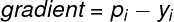
The formula for the hessian:

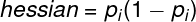
We calculate derivatives by applying the chain rule to the logloss function lwith respect to a change of an argument z.

We can imagine the process as a game of golf. A golfer (an algorithm) tries to get the ball into the hole (a correct prediction that minimizes loss); to do this, he can choose the direction and the power of the shot (the gradient) and take various clubs to get control over the strike (the hessian).

The main goal of the algorithm is to make cumulative logloss as minimal as possible (a strange golfer who chases the number of holing balls instead of making the result with minimum strikes). If we have an imbalanced dataset and features do not provide unambiguous categorization, it tends to predict that a sample belongs to the larger group (some kind of cherry-picking).

Let’s imagine a game of golf with changed rules; most holes have a standard value, but there are extras with more significant value than ordinary holes. A golfer does not understand the price of a target beforehand. If a player holes extra, he receives a higher reward. If he incorrectly identifies the hole as a standard one and refuses to approach it, he loses time and receives less compensation.

The basic algorithm cannot realize the change in rules, so it proceeds to simpler ones and fails to identify and score extras. Let’s introduce “beta” (a positive number without an upper bound) to turn the tables around. Its target is to raise a cumulative loss dramatically if the algorithm makes an incorrect cherry-picking prediction. The basic algorithm also has “beta”, which equals 1.

The beta-logloss has the following formula:

Formulas for the gradient and hessian:

The custom loss is implemented by changing the algorithm “beta” to less than 1 to penalize FN or more than 1 to make FP cost more. We should recalculate the gradient and hessian with a new “beta”, forcing the algo to change a loss calculation policy.

Let’s code custom loss

I implemented the code in scikit-learn API for XGboost in Python (version 1.0.2). We can use custom loss functions in gradient boosting packages (XGBoost, LightGBM, Catboost) or deep learning packages like TensorFlow.

There are four user-defined functions to make a custom loss function work. The first is to calculate the first derivative of the amended logloss function (a gradient), the second is to calculate the second derivative, the third is to get the objective function, and the fourth is to calculate the amended evaluation metric.

Hereafter yparameter contains an actual class value, predtgets the predicted value to evaluate.

The logreg_err_beta_sklearnfunction calculates the logloss based on the dataset for valuation. It checks performance against unseen data. Even if we apply sklearn API, this user-defined function receives dmat argument, which is DMatrix datatype (internal data structure of XGBoost).

Example based on a Titanic dataset

The titanic dataset is a case of an imbalanced dataset where the survival rate is barely 38%.

Let’s skip preprocessing steps made before modeling and go straight to the classification task. You can find a whole in my GitHub repository referenced at the end of the article.

The result of the basic algorithm is the following confusion matrix:

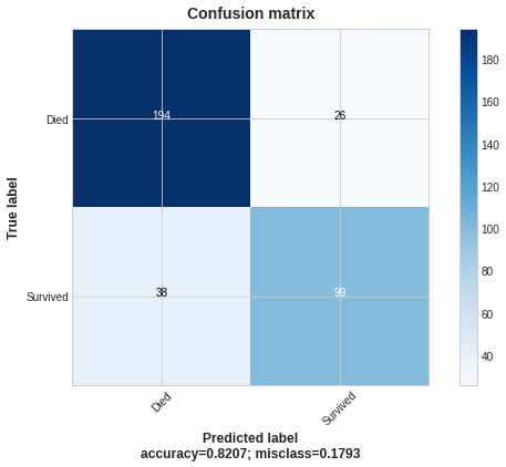
The basic algorithm gives 38 FN cases. Let’s assume that our goal is to reduce the number of FN. Let’s change an objective function to the custom one, amend evaluation metrics accordingly, and set “beta” to .4.

Changes from the basic algorithm are disabling of default evaluation metric, the explicit introduction of the custom logloss function, and the respective evaluation metric.

The confusion matrix for the beta-logloss algorithm:

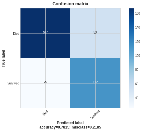
The beta algorithm decreases FN cases to 25 (-34%), true positives (TP) grew to 112 (+13%), FP grew to 53 (+103%), true negatives (TN) decreased to 167 (-14%). The fall in FN leads to a boost in both TP and FP. Overall accuracy fell.

We can easily apply the same logic to penalize FP by choosing “beta” higher than 1.

Conclusions

The beta-logloss has some distinctive pluses as well as flaws. I have listed the most obvious ones.

Advantages

• Easy and fast to apply (use four user-defined functions and beta, and that’s it).
• There is no need to perform manipulation with underlying data before modeling (if a dataset is not highly imbalanced)
• It may be applied as a part of data exploration or as a part of model stacking.
• We may add it to the most popular machine-learning packages.

Shortcuts

• We should tune “beta” to get optimal FN to FP trade-off.
• It may not provide meaningful results when a dataset is highly imbalanced (the dataset where the minor class is less than 10% of all samples). Exploratory data analysis is vital to make the model work.
• In case we penalize FN it often leads to a huge growth of FP and vice versa. You may need additional resources to compensate for that growth.

References

1. Overview of binary cross-entropy (logloss): https://towardsdatascience.com/understanding-binary-cross-entropy-log-loss-a-visual-explanation-a3ac6025181
2. Overview of the custom loss function for regression tasks: https://towardsdatascience.com/custom-loss-functions-for-gradient-boosting-f79c1b40466d
3. XGBoost documentation related to custom loss function: https://xgboost.readthedocs.io/en/latest/tutorials/custom_metric_obj.html
4. Plot_confusion_matrix function source: https://www.kaggle.com/grfiv4/plot-a-confusion-matrix
5. Link to my GitHub repository: https://github.com/kpluzhnikov/binary_classification_custom_loss

---

Outline a Smaller Class With the Custom Loss Function was originally published in Towards AI on Medium, where people are continuing the conversation by highlighting and responding to this story.

Join thousands of data leaders on the AI newsletter. It’s free, we don’t spam, and we never share your email address. Keep up to date with the latest work in AI. From research to projects and ideas. If you are building an AI startup, an AI-related product, or a service, we invite you to consider becoming a sponsor.

Published via Towards AI