Mastering Data Analysis with Pandas: A Step-by-Step Guide using Stanford Open Policing Data

Author(s): Fares Sayah

Originally published on Towards AI.

Data Analysis Project Guide — Use Pandas power to get valuable information from your data

Photo by path digital on UnsplashThe Pandas library offers a wide range of capabilities for data science, including cleaning, visualization, and exploration. However, it is important to note that just because you are using this tool does not guarantee accurate results. Improper use of the library can lead to incorrect conclusions, missed data, or misleading calculations. This tutorial will guide you through common data science tasks, showing you both how to effectively use Pandas and how to avoid common mistakes. By the end, you will have the confidence and knowledge to use Pandas in a responsible and effective manner.

This dataset contains the data obtained from the number of traffic stops made by US police and what happened during these stops. The data ranges from 2005 to 2015. The dataset was obtained from Stanford Open Policing Project. The purpose of collecting this data was to monitor and enhance the interactions between law enforcement and the public in the country.

Table of Contents:

In this project, we examine a number of factors that relate to police stopping a group of people from the Stanford region of the United States. In particular, we wish to understand the association between driver age and driver gender, as well as the time of day on police, stop them.

A good data analysis project is all about asking questions. In this blog post, we are going to answer the following questions:

1. Do men or women speed more often?
2. Does gender affect who gets searched during a stop?
3. During a search, how often is the driver frisked?
4. Which year had the least number of stops?
5. How does drug activity change by time of day?
6. Do most stops occur at night?

Read the Data

The first step is to get the data and load it to memory. You can download data from this link: Stanford Open Policing Project. We are using Pandas for data manipulation. Matplotlib, Seaborn, and hvPlot for Data Visualization. A quick way to check your data is by using .head() method.

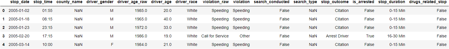
After reading the data successfully, we need to check our data. Pandas have a lot of function that allows us to discover our data effectively and quickly. The goal here is to find out more about the data and become a subject matter expert on the dataset you are working with.

In general, we need to know the following questions:

1. What kind of data do we have, and how do we treat different types?
2. What’s missing from the data, and how do you deal with it?
3. How can you add, change or remove features to get more out of your data?

Information About the Data

.info() method prints information about a DataFrame including the index dtype and columns, non-null values, and memory usage.

<class 'pandas.core.frame.DataFrame'>
RangeIndex: 91741 entries, 0 to 91740
Data columns (total 15 columns):
 #   Column              Non-Null Count  Dtype  
---  ------              --------------  -----  
 0   stop_date           91741 non-null  object 
 1   stop_time           91741 non-null  object 
 2   county_name         0 non-null      float64
 3   driver_gender       86406 non-null  object 
 4   driver_age_raw      86414 non-null  float64
 5   driver_age          86120 non-null  float64
 6   driver_race         86408 non-null  object 
 7   violation_raw       86408 non-null  object 
 8   violation           86408 non-null  object 
 9   search_conducted    91741 non-null  bool   
 10  search_type         3196 non-null   object 
 11  stop_outcome        86408 non-null  object 
 12  is_arrested         86408 non-null  object 
 13  stop_duration       86408 non-null  object 
 14  drugs_related_stop  91741 non-null  bool   
dtypes: bool(2), float64(3), object(10)
memory usage: 9.3+ MB

Descriptive Statistics about the Data

.describe() generates descriptive statistics. Descriptive statistics include those that summarize the central tendency, dispersion, and shape of a dataset’s distribution, excluding NaN values.

Analyzes both numeric and object series, as well as DataFrame column sets of mixed data types. The output will vary depending on what is provided. Refer to the notes below for more detail.

The Shape of the Data

Use ‘.shape’ to see DataFrame shape: rows, columns

(91741, 15)

Missing Values

Missing Data is a very big problem in real-life scenarios. In Pandas, missing data is represented by two values: NaN or None. Panas has several useful functions for detecting, removing, and replacing null values in Pandas DataFrame: .isna() or .isnull() used to find NaN, .dropna() used to remove NaN, and .fillna() to fill NaN with a specific value.

stop_date                 0
stop_time                 0
county_name           91741
driver_gender          5335
driver_age_raw         5327
driver_age             5621
driver_race            5333
violation_raw          5333
violation              5333
search_conducted          0
search_type           88545
stop_outcome           5333
is_arrested            5333
stop_duration          5333
drugs_related_stop        0
dtype: int64

What does NaN mean?

In computing, NaN, standing for not a number, is a member of a numeric data type that can be interpreted as a value that is undefined or unrepresentable, especially in floating-point arithmetic.

Why might a value be missing?

There are many causes of missing values, Missing data can occur because of nonresponse, Attrition, governments or private entities, …

Why mark it as NaN? Why not mark it as a 0 or an empty string or a string saying “Unknown”?

We mark missing values as NaN to make them distinguish from the original dtype of the feature.

Remove the column that only contains missing values.

stop_date           : ==============> 0.00%
stop_time           : ==============> 0.00%
county_name         : ==============> 100.00%
driver_gender       : ==============> 5.82%
driver_age_raw      : ==============> 5.81%
driver_age          : ==============> 6.13%
driver_race         : ==============> 5.81%
violation_raw       : ==============> 5.81%
violation           : ==============> 5.81%
search_conducted    : ==============> 0.00%
search_type         : ==============> 96.52%
stop_outcome        : ==============> 5.81%
is_arrested         : ==============> 5.81%
stop_duration       : ==============> 5.81%
drugs_related_stop  : ==============> 0.00%

Remove missing values: If all values are NaN, drop that row or column.

(91741, 14)

county_name All the data is missing. We will drop this column.

stop_date                 0
stop_time                 0
driver_gender          5335
driver_age_raw         5327
driver_age             5621
driver_race            5333
violation_raw          5333
violation              5333
search_conducted          0
search_type           88545
stop_outcome           5333
is_arrested            5333
stop_duration          5333
drugs_related_stop        0
dtype: int64

Do Men or Women speed more often?

To answer this question, we need to know the portion of men and women in our dataset. After that, we need to check the portion of men and women stopped for a speed violation.

M    62895
F    23511
Name: driver_gender, dtype: int64

M    0.727901
F    0.272099
Name: driver_gender, dtype: float64

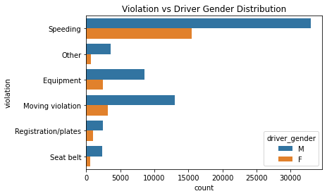
Speeding               48463
Moving violation       16224
Equipment              11020
Other                   4317
Registration/plates     3432
Seat belt               2952
Name: violation, dtype: int64

Speeding               0.560862
Moving violation       0.187760
Equipment              0.127534
Other                  0.049961
Registration/plates    0.039719
Seat belt              0.034164
Name: violation, dtype: float64

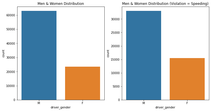1: Driver Gender Distribution — Men 62895 (73%), Women 23511 (27%) | 2: Driver Gender vs Speed Violation Distribution — Men 62895 (68%), Women 23511 (32%)

In this dataset, we 62895 (73%) Men and 23511 (27%)women. So, in responding to this question, we must take into consideration of the non-equivalent distribution of the data or use fractions.

The speeding violation represents 56% of all violations in our dataset.

M    32979
F    15482
Name: driver_gender, dtype: int64

M    0.680527
F    0.319473
Name: driver_gender, dtype: float64

When a man is pulled over, How often is it for speeding?

Speeding               32979
Moving violation       13020
Equipment               8533
Other                   3627
Registration/plates     2419
Seat belt               2317
Name: violation, dtype: int64

Speeding               0.524350
Moving violation       0.207012
Equipment              0.135671
Other                  0.057668
Registration/plates    0.038461
Seat belt              0.036839
Name: violation, dtype: float64

From 62895 Men stopped by police, 32979 (~53%) are stopped because of speeding.

When a woman is pulled over, How often is it for speeding?

Speeding               15482
Moving violation        3204
Equipment               2487
Registration/plates     1013
Other                    690
Seat belt                635
Name: violation, dtype: int64

Speeding               0.658500
Moving violation       0.136277
Equipment              0.105780
Registration/plates    0.043086
Other                  0.029348
Seat belt              0.027009
Name: violation, dtype: float64

From 23511 women stopped by police, 15482 (~66%) are stopped because of speeding.

The rate of Men stopped for speed is 68% and the rate at women stopped at speed is 32% which is different from the fraction of men (73%) and women (27%) in our data. So we can say that women are more likely to be stopped for speed violations than men.

Does Gender affect who gets searched during a stop?

To answer this question, we need to know the number of searches conducted during all stops.

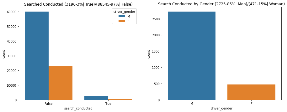
False    88545
True      3196
Name: search_conducted, dtype: int64

False    0.965163
True     0.034837
Name: search_conducted, dtype: float64

From all 88545 stoping cases, the data only 3196 (3%) are searched.

M    2725
F     471
Name: driver_gender, dtype: int64

M    0.852628
F    0.147372
Name: driver_gender, dtype: float64

Does this prove causation?

• Causation is difficult to conclude, so focus on relationships
• Include all relevant factors when studying a relationship

From the stopped cases 2725 (85%) are men and only 471 (15%)are women. This result means that men are more likely to be searched than women during a stop.

Why is ‘search_type’ missing so often?

88545

False    88545
True      3196
Name: search_conducted, dtype: int64

NaN    88545
Name: search_type, dtype: int64

search_type is missing every time the police don't search. Now we know why the search type is missing. We can fill in the missing values in the search type by Not Searched using pandas function .fillna().

Notes:

• Verify your assumptions about your data
• pandas functions ignore missing values by default

During a search, how often is the driver frisked?

search_type is a text of search types separated by commas. So, we need to separate the search type and then count the appearance of Frisk.

Incident to Arrest                                          1219
Probable Cause                                               891
Inventory                                                    220
Reasonable Suspicion                                         197
Protective Frisk                                             161
Incident to Arrest,Inventory                                 129
Incident to Arrest,Probable Cause                            106
Probable Cause,Reasonable Suspicion                           75
Incident to Arrest,Inventory,Probable Cause                   34
Incident to Arrest,Protective Frisk                           33
Probable Cause,Protective Frisk                               33
Inventory,Probable Cause                                      22
Incident to Arrest,Reasonable Suspicion                       13
Inventory,Protective Frisk                                    11
Incident to Arrest,Inventory,Protective Frisk                 11
Protective Frisk,Reasonable Suspicion                         11
Incident to Arrest,Probable Cause,Protective Frisk            10
Incident to Arrest,Probable Cause,Reasonable Suspicion         6
Incident to Arrest,Inventory,Reasonable Suspicion              4
Inventory,Reasonable Suspicion                                 4
Inventory,Probable Cause,Protective Frisk                      2
Inventory,Probable Cause,Reasonable Suspicion                  2
Incident to Arrest,Protective Frisk,Reasonable Suspicion       1
Probable Cause,Protective Frisk,Reasonable Suspicion           1
Name: search_type, dtype: int64

We will use the Counter function from collections library to count the number of each search_type.

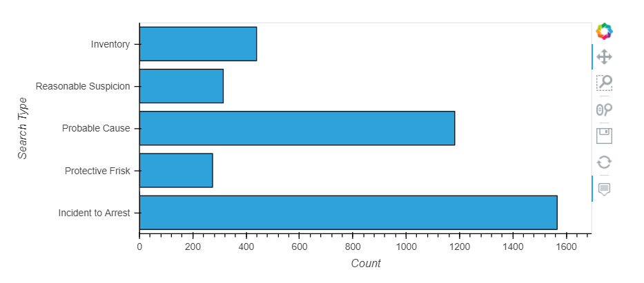
274

0.08573216520650813

We have 5 search types (Inventory, Reasonable Suspicion, Probable Cause, Protective Frisk, Incident to Arrest). From all searches conducted 247 (8.57%) are Protective Frisk.

Which year had the least number of stops?

The stop_date and stop_time are object types, so we need to convert them to Pandas DateTime objects to easily manipulate them. Having our dates as datetime64 object will allow us to access a lot of date and time information through the .dt API.

object
object

0        2005-01-02
1        2005-01-18
2        2005-01-23
3        2005-02-20
4        2005-03-14
Name: stop_date, Length: 91741, dtype: object

stop_date             datetime64[ns]
stop_time                     object
driver_gender                 object
driver_age_raw               float64
driver_age                   float64
driver_race                   object
violation_raw                 object
violation                     object
search_conducted                bool
search_type                   object
stop_outcome                  object
is_arrested                   object
stop_duration                 object
drugs_related_stop              bool
year                           int64
dtype: object

2012    10970
2006    10639
2007     9476
2014     9228
2008     8752
2015     8599
2011     8126
2013     7924
2009     7908
2010     7561
2005     2558
Name: year, dtype: int64

2012 and 2006 were the two years with the highest number of arrests by the police. 2005 was the year with the fewest arrests by the police.

How does drug activity change by time of day?

To answer this question, we need to check drug_related_stop column in our dataset, and to track these activities over the day, we use the stop_time column.

False    90926
True       815
Name: drugs_related_stop, dtype: int64

False    0.991116
True     0.008884
Name: drugs_related_stop, dtype: float64

From all the records we have, 815 (0.88%) of the stops are drug-related.

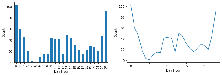
Most drug-related stops are between 10 p.m. and 1 a.m., which is very logical because most drug addicts consume drugs at this time of the day, but we need a larger dataset to confirm this assumption.

Do most stops occur at night?

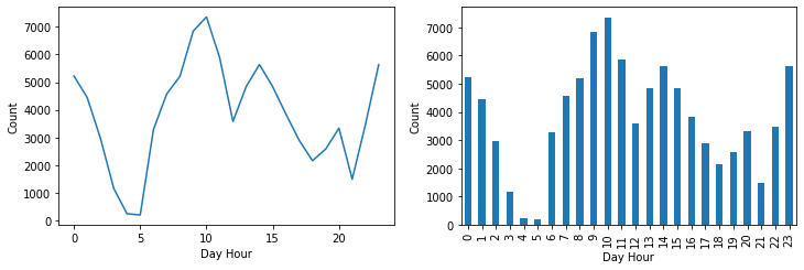
From the plots, it seems that most stops are during day time, not at night. But this is very logical because traffic in the daytime is more than traffic during nighttime.

Find the bad data in the stop_duration column and fix it

stop_duration Missing Values: 5333
stop_duration Unique Values: ['0-15 Min' '16-30 Min' '30+ Min' nan '2' '1']

By default, pandas.value_counts() ignore missing values. Pass dropna=False to make it count missing values.

0-15 Min     69543
16-30 Min    13635
NaN           5333
30+ Min       3228
2                1
1                1
Name: stop_duration, dtype: int64

It seems that we have two additional categories 1 and 2 with only one record for each. We will consider them as missing values.

0-15 Min     69543
16-30 Min    13635
NaN           5335
30+ Min       3228
Name: stop_duration, dtype: int64

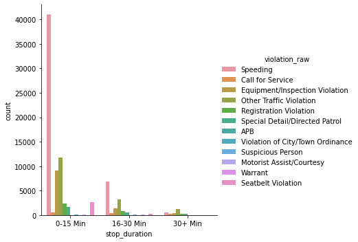
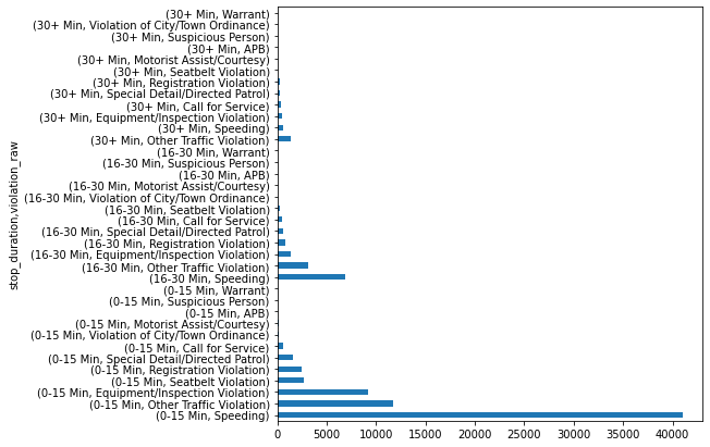
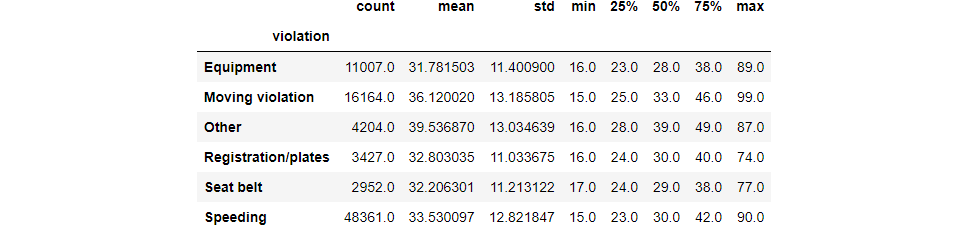
What is the mean stop_duration for each violation_raw?

For the stop_duration we have three categories: ‘0–15 Min’, ‘16–30 Min’, and ‘30+ Min’.

stop_duration Unique Values: ['0-15 Min' '16-30 Min' '30+ Min' nan '2' '1']

violation_raw Number of Unique Values: 12

violation_raw Unique Values: [
'Speeding' 'Call for Service'   
'Equipment/Inspection Violation' 
'Other Traffic Violation' 
nan 
'Registration Violation', 
'Special Detail/Directed Patrol' 
'APB' 
'Violation of City/Town Ordinance'
'Suspicious Person' 
'Motorist Assist/Courtesy' 
'Warrant'
'Seatbelt Violation'
]

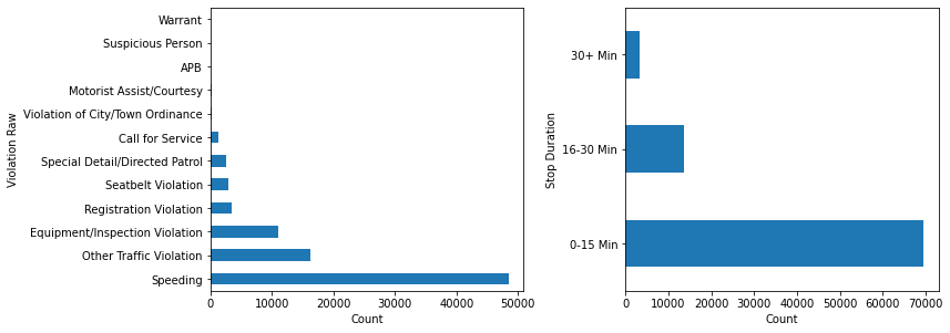
Let’s create a new column in which we replace the time intervals that we have with the mean so we can apply mathematical operations on them. we will map them as follow: ‘0–15 Min’:8, ‘16–30 Min’:23, ‘30+ Min’:45.

8.0     69543
23.0    13635
45.0     3228
Name: stop_minutes, dtype: int64

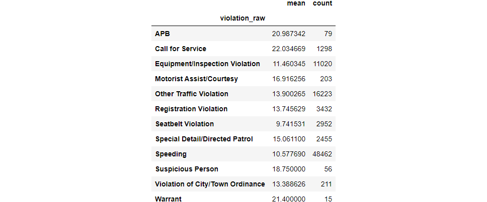
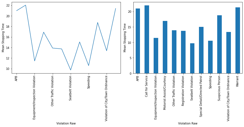
violation_raw
APB                                 20.987342
Call for Service                    22.034669
Equipment/Inspection Violation      11.460345
Motorist Assist/Courtesy            16.916256
Other Traffic Violation             13.900265
Registration Violation              13.745629
Seatbelt Violation                   9.741531
Special Detail/Directed Patrol      15.061100
Speeding                            10.577690
Suspicious Person                   18.750000
Violation of City/Town Ordinance    13.388626
Warrant                             21.400000
Name: stop_minutes, dtype: float64

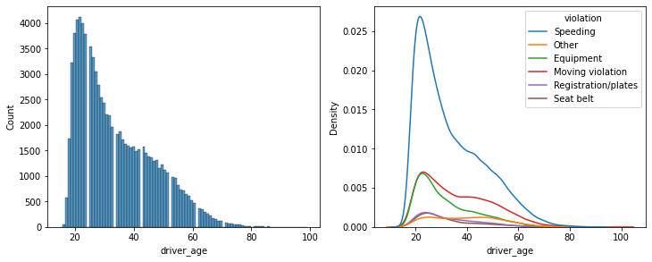
Compare the age distributions for each violation

Summary

Good data analysis requires both mastering the tools (Python and Pandas) and Creative thinking (Understanding the problem we are solving and asking the right questions). In this article, we discovered how to perform data analysis. Specifically, we learned:

• One of the first steps when exploring a new data set is making sure the data types are set correctly.
• Causation is difficult to conclude, so focus on relationships. So, Include all relevant factors when studying a relationship.
• Use the DateTime data type for dates and times.
• Use visualization tools to help you understand trends in your data.

Links and Resources:

• Link to data used in this tutorial: Stanford Open Policing Project
• Link to Full Notebook

---

Mastering Data Analysis with Pandas: A Step-by-Step Guide using Stanford Open Policing Data was originally published in Towards AI on Medium, where people are continuing the conversation by highlighting and responding to this story.

Join thousands of data leaders on the AI newsletter. Join over 80,000 subscribers and keep up to date with the latest developments in AI. From research to projects and ideas. If you are building an AI startup, an AI-related product, or a service, we invite you to consider becoming a sponsor.

Published via Towards AI