Author(s): Mishtert T

Originally published on Towards AI.

Simple Linear Regression

Customer Lifetime Value (CLV)

In marketing, customer lifetime value (CLV or often CLTV), lifetime customer value (LCV), or lifetime value (LTV) is a prediction of the net profit attributed to the entire future relationship with a customer. Wikipedia

Why do we need to know or understand about CLV?

• CLV describes the ‘predicted future net-profit ’ accumulated by a company through its relationship with the customer.
• Helps in identifying potential promising customers who will generate a higher net profit
• Helps in targeting or prioritizing customers according to future margins

Net profit, also known as margins, is the metric of interest. For this reason, we have to find the drivers affecting the magnitude of the margin.

There is one tricky aspect of this. We have to predict the future margin using the only data that is available at that time. Hence we need a model that uses the current information to predict the future margin.

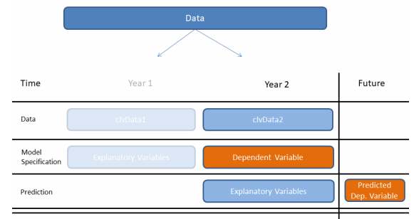
Two-Step Procedure.

We have to apply a two-step procedure. We have to take the explanatory variables from Year 1 and use them to predict the dependant variable for Year 2. We call this model specification.

After specifying the model, we’ll take the explanatory variables from Year 2 and make predictions for future margins of Year 3

Typical CLV Dataset

Finding Relationships

First, we should find a relationship between Year 1 variables and predicted futureMargin.

We can find correlation from cor() function in stats package and create a correlation plot using corrplot() function from corrplot package to visualize the relationship

library(corrplot)
 
clv_data1 %>% 
 select(nOrders, nItems, ... margin, futureMargin) %>%
 cor() %>%
 corrplot()

Notice the strong positive relationship between, plotted in Blue:

• The number of ordersnOrders,
• The number of items nItems
• The future marginfutureMargin

We find a somewhat stronger positive correlation between the current year margin and futureMargin.

The daySinceLastOrder and the returnRatio are moderately negatively correlated with the futureMargin, plotted in orange.

Simple Linear Regression

Now that we’ve inspected the correlations of various variables, we’ll move on to predicting future margins with the help of the margin in Year 1.

Now that we have examined the correlations of various variables, we will proceed to estimate future margins with the help of the Year 1 margin.

We chose margin because the correlation between the two variables is the highest.

When we use only one independent variable for prediction, we call the model a simple linear regression.

In reality, the ideal case of a perfect linear correlation, where we can exactly predict Y with the given value of X is very unlikely.

Most of the time, the data points are scattered around. We determine the direction of the relationship between X and Y by fitting a straight line through the scattered data points.

We use the Least Square Estimation (LSE) procedure to helps us find the regression line and return its coefficients.

The difference between the prediction, a point on the line, and the actual value, a data point on the scattered data points, is called prediction error or residual value.

We can specify the linear regression order using a formula object in the lm function in the stats package.

slm <- lm(futureMargin ~ margin, data = clv_data1) 
summary(slm)

Notice that we are going to predict future margin as a function of margin using clv data. We store the model as slm, then we use the summary function to get an overview of the results.

Looking at the coefficient estimate for the margin, with a value of roughly 0.65 (it is greater than ‘zero’), means that higher the margin in the higher we expect the future margin to be.

Also, take a look at the Multiple R-squared, a value of ~0.32 means, that the margins in the can explain about 30% of the variation in the future margin Year 1.

Visualization of Relationship

The below ggplot representation gives us a better view of the relationship between year 1 margin and year2 margin

ggplot(clv_data1,aes(margin,futureMargin)) +
geom_point() +
geom_smooth(method=lm,se=FALSE) +
xlab("Marginyear1") +
ylab("Marginyear2")

There are some assumptions that we make if we are to use the linear regression modeling method.

Assumptions (Simple Linear Regression Model)

• A linear relationship between the dependent variable and independent variable.
• The independent variable should not contain any measurement errors(weak exogeneity)
• The residuals should be uncorrelated
• The residuals should randomly vary around zero, and their expectation should be equal to zero
• The variance of the prediction errors should be constant(homoscedasticity)
• When doing statistical significance testing, we have to assume that the errors are normally distributed

To be continued…

Let’s look at how to predict the future margin better using Multiple Linear Regression modeling in the next article.

Join thousands of data leaders on the AI newsletter. Join over 80,000 subscribers and keep up to date with the latest developments in AI. From research to projects and ideas. If you are building an AI startup, an AI-related product, or a service, we invite you to consider becoming a sponsor.

Published via Towards AI