Machine Learning: The First Step is to Understand Simple Linear Regression

Author(s): Dede Kurniawan

Originally published on Towards AI.

Mastering Simple Linear Regression in Python without a Lot of Math

In the machine learning universe, who doesn’t know about linear regression? Of course, everyone knows about it. Linear regression is the most fundamental and widely applied concept in daily life. Simple linear regression is used to find the correlation between two variables (explanatory and response variables). In addition, linear regression aims to predict the value of the response variable from the value of the explanatory variable that has never been observed before [1].

I will explain simple linear regression using a little math in this article. The goal is that you can understand how it works and how to apply it using Python.

Get an intuition of simple linear regression

Linear regression works by drawing a line that is as close as possible to the existing data points [2]. The data points are the values of the explanatory and response variables. Simple linear regression assumes that the two explanatory and response variables are linearly correlated so that a straight line can be drawn.

How do we get the regression line? 1) The first step is to randomly select a straight line. 2) Next, randomly select data points and adjust the line as close as possible to each data point. 3) Repeat the second step several times until you get a line that is as close as possible to all data points [2].

Let’s imagine we have a collection of student data containing the study duration and the score obtained during the exam. We are asked to predict the students’ scores from their study duration. Let’s try to apply simple linear regression thinking to this problem.

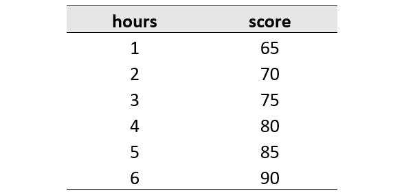
Based on the information from the data, what is the score if a student studies for 7 hours? The answer is 95. You may realize that the longer the study duration, the better score they will get. From the pattern of the data, we can conclude that for every 1 hour of study duration, they get a score of +5. We can think that the score is obtained from a combination of two things: the score obtained by students with <1 hour of study duration and the score obtained by students while studying. Let’s simplify it using a formula:

What we have here is a formula to predict the score that students get from their study duration. Using the formula, we can predict that a student who studies for 7 hours will most likely get a score of 95.

The formula we get is the same as the formula in simple linear regression. In simple linear regression, the formula is like this:

Yes, the simple linear regression formula has actually been learned in middle school. Back then, we probably only used it to find the gradient of a straight line. In simple linear regression, the formula means the following:

• y → the response/target variable that we are trying to predict from the explanatory variables. In the above problem, this is the “score”.
• x → the explanatory variable we are using to make a prediction. In the problem above, this is “hours”.
• m → Slope is the steepness of the regression line that tells us how much we expect the y value to increase when we increase the x value by one unit. In machine learning, the slope is also known as weight.
• c → The intercept tells us where the regression line crosses the vertical y-axis. In machine learning, the intercept is also known as bias.

Next, how do we know how well our regression line fits the data points? The answer is to minimize the error in the model prediction to find the best line. Defining and measuring the error of a model is called loss function or cost function sometimes also called error function. The difference between the predicted value and the observed value is called the residual (error). The measure of the fit of a model to predict all values of the response variable close to the observed values is called the residual sum of squares (RSS/SSres) [1].

Perform simple linear regression using Python

After getting an intuition about the concept of simple linear regression, we will proceed by performing simple linear regression using Python. You can download the dataset that we will use on Kaggle. There are some libraries that we need to import first that can make it easier for us when building a simple regression model.

import numpy as np
import pandas as pd
import matplotlib.pyplot as plt

Next, we can read and load the dataset using Pandas.

# read and load the data
df = pd.read_csv("score.csv")
df.head()

# get information about the data
df.info()

# output
<class 'pandas.core.frame.DataFrame'>
RangeIndex: 25 entries, 0 to 24
Data columns (total 2 columns):
 # Column Non-Null Count Dtype 
--- ------ -------------- ----- 
 0 Hours 25 non-null float64
 1 Scores 25 non-null int64 
dtypes: float64(1), int64(1)
memory usage: 528.0 bytes

# data preparation
from sklearn.model_selection import train_test_split

X = df.iloc[:,:-1].values
y = df.iloc[:, 1:].values
X_train, X_test, y_train, y_test = train_test_split(X, 
 y, 
 test_size=0.3,
 random_state=99)

The data set has two columns, “Hours” and “Scores”. The “Hours” column will be the explanatory variable, while the “Scores” column will be the response variable. In addition, the dataset only consists of 25 rows and no missing values. We also need to separate the data set into training and test data. The training data is used to build a simple regression model, while the test data is used to evaluate how good our model is. Now is the time to build the regression model!

# build regression model
from sklearn.linear_model import LinearRegression

model_reg = LinearRegression()
model_reg.fit(X_train, y_train)

To build and train a simple regression model, we can use Scikit-learn. To see the fit of the regression model to the data set, we can visualize it using Matplotlib.

# visualize the regression model
X_vis = np.array([0, 10]).reshape(-1, 1)
y_vis = model_reg.predict(X_vis)
plt.scatter(X_train, y_train, label="Actual values")
plt.plot(X_vis, y_vis, "-r", label="Regression line")
plt.title("Regression analysis")
plt.ylabel("Score")
plt.xlabel("Hours")
plt.xlim(0, 10)
plt.ylim(0, 100)
plt.legend()

The simple regression model seems to be pretty good at drawing a line linearly between a set of data points. As we discussed above, the linear regression formula is as follows:

To know the value of the regression equation produced by the model, we must display the intercept and slope values.

# input
print(f'intercept: {model_reg.intercept_}')
print(f'slope: {model_reg.coef_}')

# output
intercept: [1.91863322]
slope: [[9.82609393]]

From the intercept and slope values, we can know that the regression equation produced by the model is y = 9.82609393X + 1.91863322. To confirm the results of the slope and intercept values from Scikit-learn, we can also calculate these values using the equation.

# calcullate the slope value
cov_xy = np.cov(X_train.flatten(), y_train.flatten())
variance_x = np.var(X_train, ddof=1)
slope = cov_xy[0][1] / variance_x

# calcullate the intercept value
intercept = np.mean(y_train) - slope * np.mean(X_train)

print(f"slope: {slope}")
print(f"intercept: {intercept}")
print(f"regression formula: y = {slope} X + {intercept}")

It turns out that the intercept and slope values we calculated are the same as the values from Scikit-learn. Then, we also have to evaluate how good the regression model is. One of the standard metrics for evaluating linear regression models is R-squared (R²) [3].

# evaluate the regression model
from sklearn.metrics import r2_score

y_pred = model_reg.predict(X_test)
r_squared = r2_score(y_test, y_pred)
print(f'R-squared: {r_squared}')

# ouput
R-squared: 0.9230325919412203

The R² value of 0.9230325919412203 indicates that the regression model we have built is quite good. The R² value is in the range of 0 to 1, the accuracy of the regression model is getting better if the R² value is close to 1 [4]. To ensure the R² value generated by Scikit-learn, we can calculate it using the R² formula.

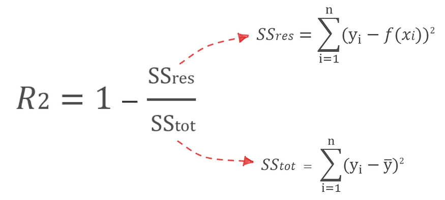
# calcullate the r-aquared value
ss_res = sum([(y_i - model_reg.predict(x_i.reshape(-1, 1))[0])**2
 for x_i, y_i in zip(X_test, y_test)])
ss_tot = sum([(y_i - np.mean(y_test))**2 for y_i in y_test])
r_squared = 1 - (ss_res / ss_tot)

print(f'R-squared: {ss_res} / {ss_tot} = {r_squared}')

# output
R-squared: [250.45194582] / [3254.] = [0.92303259]

Our results show the same R² value as the calculation from Scikit-learn. We can also use other evaluation metrics such as MAE, MSE, and MAPE to check how well our regression model is.

Conclusion

Simple linear regression is the most fundamental concept of machine learning. It works by randomly initiating a line, fitting the line to each data point, and obtaining a line that is as close as possible to the entire data point. Besides being used to determine the correlation between data, simple linear regression can also be used to make predictions. A commonly used metric to evaluate how good a linear regression model is is R-squared (R²).

References:

[1] Hackeling, G. (2017). Mastering Machine Learning with Scikit-Learn. Packt Publishing.

[2] Serrano, L. (2021). Grokking Machine Learning. Manning Publications.

[3] Chicco, D., Warrens, M., & Jurman, G. (2021). The coefficient of determination R-squared is more informative than SMAPE, MAE, MAPE, MSE and RMSE in regression analysis evaluation. PeerJ Computer Science.

[4] Al-Mosawe, A., Kalfat, R., & Al-Mahaidi, R. (2017). Strength of Cfrp-steel double strap joints under impact loads using genetic programming. Composite Structures.

Join thousands of data leaders on the AI newsletter. Join over 80,000 subscribers and keep up to date with the latest developments in AI. From research to projects and ideas. If you are building an AI startup, an AI-related product, or a service, we invite you to consider becoming a sponsor.

Published via Towards AI