Logistic Regression Math Deduction

Author(s): Fernando Guzman

Originally published on Towards AI the World’s Leading AI and Technology News and Media Company. If you are building an AI-related product or service, we invite you to consider becoming an AI sponsor. At Towards AI, we help scale AI and technology startups. Let us help you unleash your technology to the masses.

Logistic regression is a supervised machine learning algorithm to create models used for binary classification problems conventionally. Even that in its name, it says regression. This algorithm is used to train models for classification problems.

This model has also considered the first representation of an artificial neuron given that its workflows simulate a neuron where there is an array with the input values and the bias, and they are weighted by the parameters that give as a result something known as the logit normally represented by Z, and this result is passed through a sigmoid function to obtain the prediction, as in the following image:

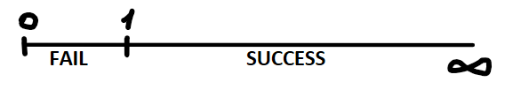
The hermeneutics of this algorithm is the same as linear regression but with an additional step which we will explain later. This algorithm is based on the Bernoulli distribution that models just two possible cases, which are success or failure, and this is also the reason why logistic regression is used to solve binary classification problems, given that there are only two possible outputs. Let’s illustrate this:

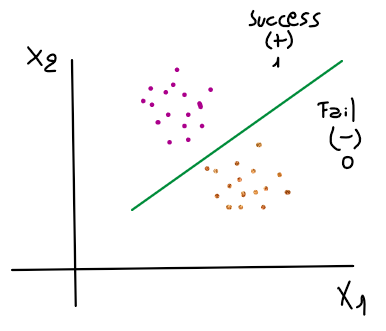
Then, to set up a clear concept of logistic regression, we will understand this model as a line that tries to identify a separation line in the data that can have only two possible outputs. Now we have a global idea of logistic regression algorithms, and we are ready to get into the math deduction of this algorithm. For this purpose, we need to understand that the hermeneutics of this algorithm is the same as linear regression. It only has an extra step which is the logit, that changes a little bit all the equations used in the process of training the model.

LOGIT

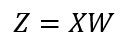
In simple terms, logits in logistic regression are the prediction of linear regression, which is represented by the following expression:

Then, let’s explain the deduction of how we get the logits. First, we need to understand the difference between two core concepts, which are probability and odds, because many people confuse them as if they are the same. A probability is how likely is an event going to happen, and the odd is the proportion between the probability of success and failure. Take as an example a coin toss. The probability of getting a head or tail is 50% or 0.5; The odds on the other hand, are given by the following expression:

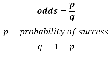
Where p represents the probability of success and q is the complement of the probability. So, given this expression, we would assume that the odds in the coin toss example would be the following:

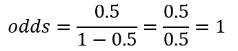
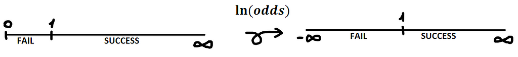
Now that we know the difference between odds and probabilities, we are ready to move on. The deductions for logits start off at the odds expression because p is the probability of success and the complement is the probability of failure, but as you might notice, this expression is a non-linear function which have not the same range of outputs as shown in the following picture:

See that the possibility of each output is not equally distributed. To solve this, we need to make the odds expression a linear function by applying the natural logarithm function. That way, we reach an equal distribution of the possibilities:

Now, we have the possibilities equally distributed, and this is actually the logit, but in the case of logistic regression, we simply take the probability as the prediction or y_hat, which can only have two possible answers, 0 or 1. Then, let’s have a look at the following expression, which represents the logit:

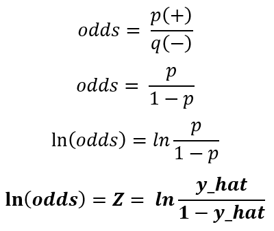
Now we have the logit expression, but you might be wondering that this expression is not the same expression as linear regression prediction, which we said was the logit at the beginning. Well, it turns out that it is the same expression, and its as follows:

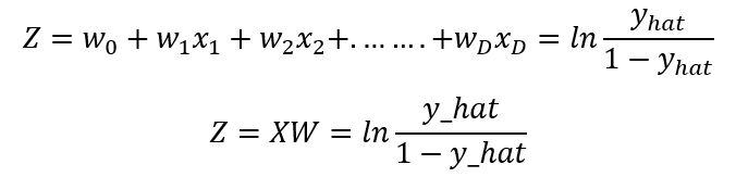
Now we have the deductions for the logits, we can move forward to the prediction but keep in mind this expression as we need it for the prediction’s deduction.

PREDICTION

The prediction function is essentially the sigmoidal function, this comes up from applying the exponential function to the logit expression and making some math operations which are in the deduction below:

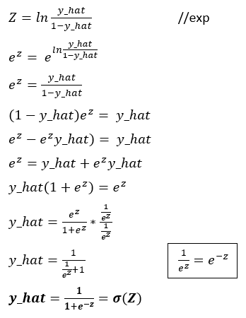
As you can see, after applying the exponential function, the exponential of Z or the logit becomes the original function of the odds because exponential and logarithmic functions is opposites, then we perform some algebra operations to finally end up in the sigmoidal function of Z which is the prediction for logistic regression.

LOSS FUNCTION

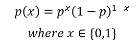
In this case, to measure the error rate we will use the maximum likelihood method, which is very convenient given that we are using a binary classification algorithm based on the Bernoulli distribution because the deduction for maximum likelihood starts off with the Bernoulli distribution as well, so let’s have a look at the Bernoulli’s formula:

For logistic regression, we set this formula by assuming p as the prediction and x are the possible outputs y given a set of data x as in the following:

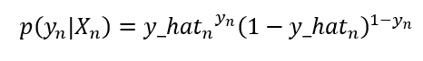
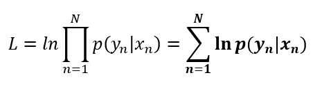
This is the probability expression for a single register in the logistic regression. We can generalize this expression as the product of all probabilities of the data set as follow:

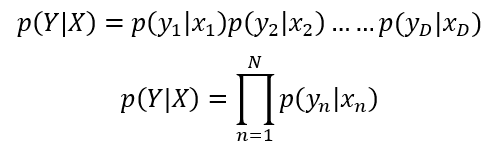
The expression we just deducted is the likelihood of the dataset, but as you may have seen, this expression is very difficult to compute while the dataset increases in size. To solve this, we need to minimize the expression using the logarithmic function, and we end up with the following expression:

Now, you can see that this is simpler to compute, and if we replace the Bernoulli formula for logistic regression in this expression, we will get to the likelihood formula. So, let’s make the deduction:

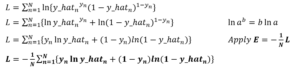
We made it!!, we have the formula of maximum likelihood to measure the error in our model training.

GRADIENT DESCENT

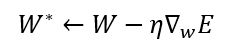
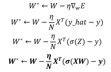
Now we have almost all the elements to train our logistic regression model, but there is still left the gradient descent which we will use to optimize the vector parameters of our model. The gradient descent formula is given by:

This is clearly the same gradient descent used for parameter optimization of any model, but the difference is in the gradient of the error. To see which is the real formula of gradient descent for logistic regression, we need to find the gradient of the error, in this case, the gradient of the maximum likelihood, which can be found using the chain rule:

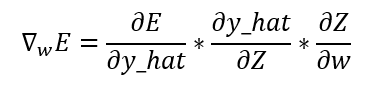
Following this method, we need to get the derivatives of the error, the prediction, and the logits. So, let’s get them:

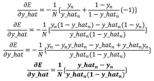
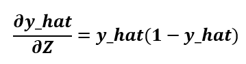
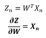
Notice that the prediction derivative ends up being the same as the sigmoidal derivative, and the logit derivative can be found directly from the logit formula. Now that we have the three necessary derivatives let’s replace them in the chain rule to get the gradient of the maximum likelihood:

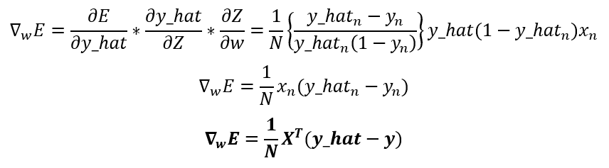
As you can see, the gradient of the error stills looks like the gradient of the linear regression, but in this case, have into account that the prediction is a different function, and that’s the only thing that makes the logistic regression gradient different from the linear regression.

Now that we have the gradient let’s see the gradient descent for logistic regression, which is represented by the following expression:

In the linear regression, we also mentioned that there is also the direct method to optimize the parameters; This is not the case for logistic regression. The direct method cannot be used for this algorithm optimization, the only method available is the gradient descent.

LOGISTIC REGRESSION IMPLEMENTATION

We are now set with all the elements to understand the full implementation and training of a logistic regression model, so let’s have a look at the next illustration:

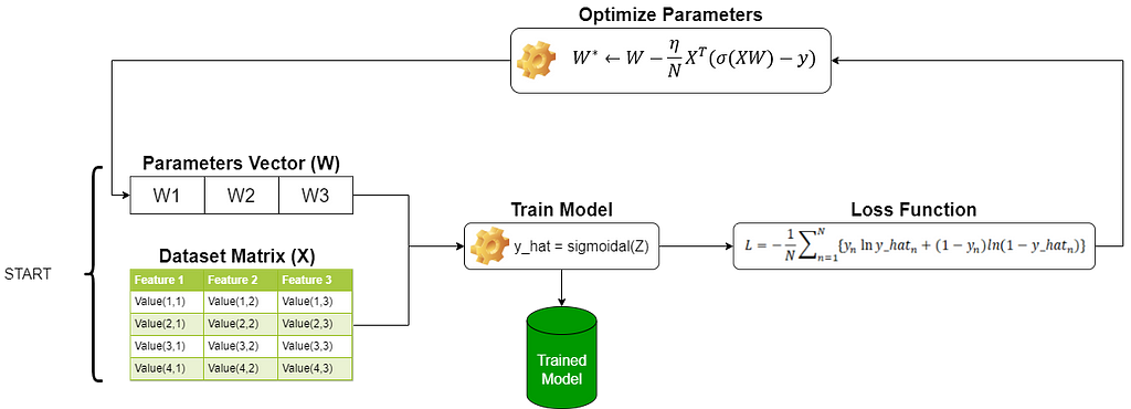
As you can see, the process is still the same as linear regression where we have a matrix dataset as input and a vector parameter randomly started; These inputs are operated by the prediction function, then we measure our error with the loss function then based on this result we optimize the parameters vector with the gradient descent but in this case, the prediction is given by other equation. Also, notice that we have used the maximum likelihood as the loss function compared to the linear regression article, where we used the minimum square error as the loss function. Keep in mind that the loss function and the gradient descent both use the prediction in their expressions; So, as the prediction function has changed, both equations have also changed because of the prediction function.

SOFTMAX REGRESSION

There is also another machine learning algorithm called softmax regression or multiclass logistic regression. This is an extension of the traditional binary logistic regression; This version defines the idea of having multiple results. The process is essentially the same. To not make this long, we will only see its differences.

Traditional logistic regression has only one logit because the prediction can provide only two possible outputs, in this case, we have many outputs, which are called classes, and for each of them, we have a logit and a prediction which is a probability; Then, we can assume that our final output will be a vector of probability values where the selected answer will be the class with the highest probability, like in the next illustration:

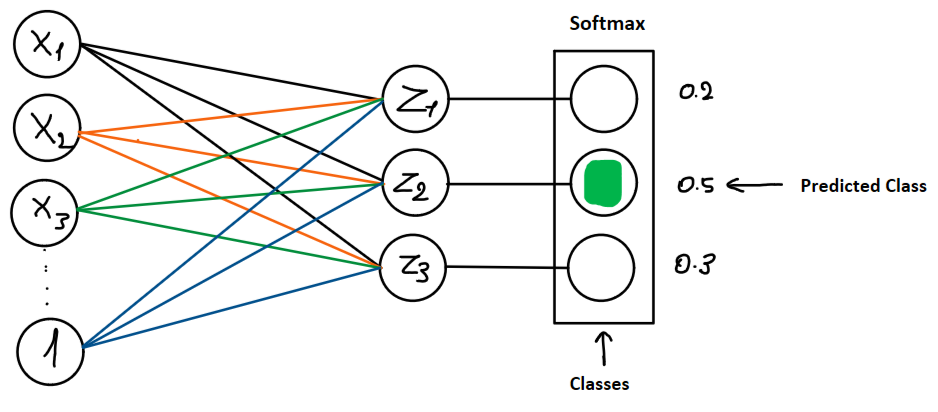
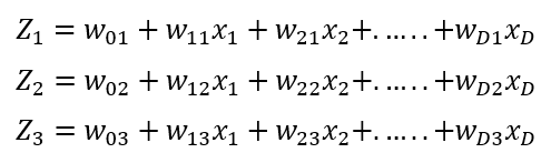
In this illustration, we can see that the parameters are no longer a vector, instead, we have a matrix of parameters; This is what allows us to generate a logit for each given class represented as the following expression:

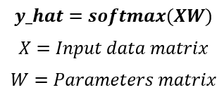
In the binary logistic regression, after the logit was computed, we operated this result with a sigmoidal function; In the case of softmax regression, after the logit is obtained, we compute each logit with a softmax function instead of a sigmoidal, this is the reason why this version is called softmax regression. So, let’s see how softmax is represented in its mathematical form:

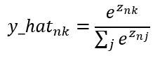
As you can see, softmax is our prediction and is given by this equation where n is the number of registers or rows, k is the number of classes and Z is our logit. To resume, this operation to get the prediction compared to binary logistic regression where we have a vector and a matrix product change to a two-matrix product and computed with a softmax function, like the following:

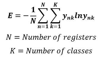
Something else that changes in this version is the loss function. We have deducted the maximum likelihood to measure the error of the binary logistic regression. This function is also known as binary cross-entropy. In the case of softmax regression, there is also an extension of this equation to work as the loss function, which is called categorical cross-entropy. This function is given by the following expression:

Having these changes in mind, you will be able to implement the softmax regression with the same process of binary logistic regression.

I hope this was very useful for you!!

---

Logistic Regression Math Deduction was originally published in Towards AI on Medium, where people are continuing the conversation by highlighting and responding to this story.

Join thousands of data leaders on the AI newsletter. It’s free, we don’t spam, and we never share your email address. Keep up to date with the latest work in AI. From research to projects and ideas. If you are building an AI startup, an AI-related product, or a service, we invite you to consider becoming a sponsor.

Published via Towards AI