Logistic Regression: Intuition & Implementation

Author(s): Muhammad Arham

Originally published on Towards AI.

The math behind the Logistic Regression algorithm and implementation from scratch using Numpy.

Introduction

Logistic Regression is a fundamental binary classification algorithm that can learn a decision boundary between two different sets of data attributes. In this article, we understand the theoretical aspect behind the classification model and implement it using Python.

Intuition

Dataset

Logistic Regression is a supervised learning algorithm so we have data feature attributes and their corresponding labels. The features are independent variables, denoted by X, and are represented in a one-dimensional array. The class labels, denoted by y, are either 0 or 1. Therefore, Logistic Regression is a binary classification algorithm.

If the data has d-featuers:

Cost Function

Similar to Linear Regression, we have associated weights for the feature attributes and a bias value.

Our aim is to find the optimal values for the weights and bias, to fit our data better.

We have a weight value associated with each feature attribute and a single bias value.

We randomly initialize these values and optimize them using Gradient Descent. During training, we take a dot product between weights and features and add the bias term.

But because our target labels our 0 and 1, we use a non-linear Sigmoid function, represented by g, that pushes our values between the required range.

The sigmoid function plotted is as follows:

Logistic Regression aims to learn weights and bias such that the values passed to the sigmoid function are positive for positive labels and negative for negative labels.

To predict values in Logistic Regression, we pass our predictions to the sigmoid function. So, the prediction function is:

Now that we have predictions from our model, we can compare them with the original target labels. The error between the predictions is calculated using the Binary Cross Entropy Loss. The loss function is as follows:

where y is the original target label, and p is the predicted value between [0,1]. The loss function aims to push the predicted values toward the actual target labels. If the label is 0 and the model predicts 0, the loss is 0. Similarly, if both predicted and target labels are 1, the loss is 0. Else, the model tries the converge to these values.

Gradient Descent

We use the Cost function and obtain the derivative concerning weights and bias. Using chain rule and mathematical derivation, the derivatives are as follows:

We obtain a scalar value that we can use to update the weights and biases.

This updates the values against the loss gradient, so after multiple iterations, we gradually converge toward the optimal values of weights and biases.

During inference, we can then use the weights and bias values to obtain predictions.

Implementation

We utilize the mathematical formulas mentioned above to code the Logistic Regression model and will evaluate its performance on some benchmark datasets.

Firstly, we initialize the class and parameters.

class LogisticRegression():
 def __init__(
 self,
 learning_rate:float=0.001,
 n_iters:int=10000
 ) -> None:
 self.n_iters = n_iters
 self.lr = learning_rate
 
 self.weights = None
 self.bias = None

We require the weights and bias values that will be optimized, so we initialize them here as object attributes. However, we can not set the size here as it depends on the data passed during training. Thus, we set them to None for now. The learning rate and number of iterations are hyperparameters that can be tuned for performance.

Training

def fit(
 self,
 X : np.ndarray, 
 y : np.ndarray
 ):
 n_samples, n_features = X.shape
 
 # Initialize Weights and Bias with Random Values
 # Size of Weights matirx is based on the number of data features
 # Bias is a scalar value
 self.weights = np.random.rand(n_features)
 self.bias = 0
 
 for iteration in range(self.n_iters):
 
 # Get predictions from Model
 linear_pred = np.dot(X, self.weights) + self.bias
 predictions = sigmoid(linear_pred)
 
 loss = predictions - y
 
 # Gradient Descent based on Loss
 dw = (1 / n_samples) * np.dot(X.T, loss)
 db = (1 / n_samples) * np.sum(loss)
 
 # Update Model Parameters
 self.weights = self.weights - self.lr * dw
 self.bias = self.bias - self.lr * db

The training function initializes the weights and bias values. We then iterate over the dataset multiple times, optimizing these values towards convergence, such that the loss minimizes.

Based on the above equations, the sigmoid function is implemented as follows:

def sigmoid(x):
 return 1 / (1 + np.exp(-x))

We then use this function to generate predictions using:

linear_pred = np.dot(X, self.weights) + self.bias
predictions = sigmoid(linear_pred)

We calculate loss over these values and optimize our weights:

loss = predictions - y
 
# Gradient Descent based on Loss
dw = (1 / n_samples) * np.dot(X.T, loss)
db = (1 / n_samples) * np.sum(loss)

# Update Model Parameters
self.weights = self.weights - self.lr * dw
self.bias = self.bias - self.lr * db

Inference

def predict(
 self,
 X : np.ndarray,
 threshold:float=0.5
 ):
 linear_pred = np.dot(X, self.weights) + self.bias
 predictions = sigmoid(linear_pred)
 
 # Convert to 0 or 1 Label 
 y_pred = [0 if y <= threshold else 1 for y in predictions]
 
 return y_pred

Once we have fit our data during training, we can use the learned weights and bias to generate predictions similarly. The output of the model is in the range [0, 1], as per the sigmoid function. We can then use a threshold value such as 0.5. All values above this probability our tagged as positive labels and all values below this threshold our tagged as negative labels.

Complete Code

import numpy as np


def sigmoid(x):
 return 1 / (1 + np.exp(-x))

class LogisticRegression():
 def __init__(
 self,
 learning_rate:float=0.001,
 n_iters:int=10000
 ) -> None:
 self.n_iters = n_iters
 self.lr = learning_rate
 
 self.weights = None
 self.bias = None
 
 def fit(
 self,
 X : np.ndarray, 
 y : np.ndarray
 ):
 n_samples, n_features = X.shape
 
 # Initialize Weights and Bias with Random Values
 # Size of Weights matirx is based on the number of data features
 # Bias is a scalar value
 self.weights = np.random.rand(n_features)
 self.bias = 0
 
 for iteration in range(self.n_iters):
 
 # Get predictions from Model
 linear_pred = np.dot(X, self.weights) + self.bias
 predictions = sigmoid(linear_pred)
 
 loss = predictions - y
 
 # Gradient Descent based on Loss
 dw = (1 / n_samples) * np.dot(X.T, loss)
 db = (1 / n_samples) * np.sum(loss)
 
 # Update Model Parameters
 self.weights = self.weights - self.lr * dw
 self.bias = self.bias - self.lr * db
 
 
 def predict(
 self,
 X : np.ndarray,
 threshold:float=0.5
 ):
 linear_pred = np.dot(X, self.weights) + self.bias
 predictions = sigmoid(linear_pred)
 
 # Convert to 0 or 1 Label 
 y_pred = [0 if y <= threshold else 1 for y in predictions]
 
 return y_pred

Evaluation

import numpy as np
import matplotlib.pyplot as plt

from sklearn.model_selection import train_test_split
from sklearn.datasets import load_breast_cancer
from sklearn.metrics import accuracy_score

from model import LogisticRegression


if __name__ == "__main__":
 data = load_breast_cancer()
 X, y = data.data, data.target
 
 X_train, X_test, y_train, y_test = train_test_split(X, y, test_size=0.2, shuffle=True)
 
 model = LogisticRegression()
 model.fit(X_train, y_train)
 y_pred = model.predict(X_test)
 score = accuracy_score(y_pred, y_test)
 
 
 print(score)

We can use the above script to test our Logistic Regression model. We use the Breast Cancer dataset from Scikit-Learn for training. We can then compare our predictions with the original labels.

Carefully fine-tuning some of the hyperparameters gave me an accuracy score of above 90%.

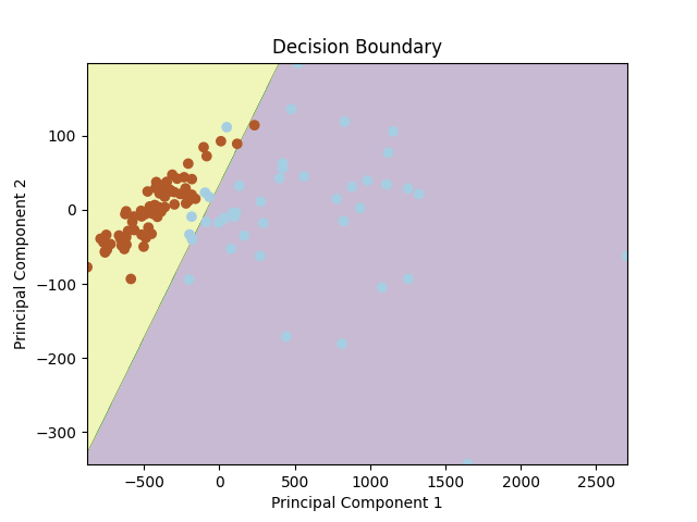
We can use different dimensionality reduction techniques such as PCA, to visualize the decision boundary. After reducing our features to two dimensions, we obtain the following decision boundary.

Conclusion

In conclusion, this article explored the mathematical intuition of Logistic Regression and demonstrated its implementation using NumPy. Logistic Regression is a valuable classification algorithm that utilizes the sigmoid function and gradient descent to find an optimal decision boundary for binary classification.

For code and implementation, refer to this GitHub repo. Follow me for more articles on deep learning architectures and research advancements.

Join thousands of data leaders on the AI newsletter. Join over 80,000 subscribers and keep up to date with the latest developments in AI. From research to projects and ideas. If you are building an AI startup, an AI-related product, or a service, we invite you to consider becoming a sponsor.

Published via Towards AI