Linear Models for Classification, Logistic Regression, with&without sklearn library

Last Updated on July 30, 2021 by Editorial Team

Author(s): Ibrahim Kovan

Machine Learning

This article deductively breaks down the topic of logistic regression, which is linear models for classification. It explains how the Logistic Regression algorithm works mathematically, how it is implemented with the sklearn library, and finally how it is implemented in python with mathematical equations without the sklearn library. Furthermore, multiclass classification for linear models is explained.

Table of Contents (TOC)
---- Introduction
---- Linear Models for Classification without Sklearn
---- Linear Models for Classification with Sklearn
-----Linear Models for Multiclass Classification

Introduction

Linear models are used for classification as well as regression. One of them, Logistic Regression, is used for binary classification as opposed to its name. Binary classification means that the dataset includes 2 outputs(classes). In addition, Logistic Regression is the fundamental part of Neural Networks. It works on minimizing the error(cost) in each iteration by updating the initial values set by the user. Figure 1 shows the flowchart of how the dataset with 4 features and 2 classes is classified with logistic regression.

1. In the training part of logistic regression, 1 weight is assigned for each feature and 1 bias value is added to the system.
2. These weights and bias values are initialized with values selected by the user.
3. Each weight is multiplied by the own feature values and added by adding the bias value.
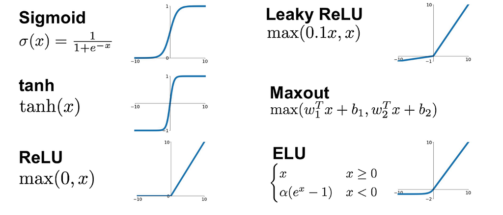
4. The activation function (figure 2) which is chosen by the user is applied to the sum value.
5. When we assume that it was a sigmoid function, Activation Function(sum) will become between 0–1 and the error is calculated by this value.
6. According to the calculated error value, the weights and bias values are updated with gradient descent (click here) at the rate of learning rate.
7. This process is repeated as many as the number of iterations. Now, let’s implement the above-mentioned processes on the breast cancer dataset with codes.

Linear Models for Classification without Sklearn library

Dataset is imported and feature values are normalized with MinMaxScaler and the data is separated with train_test_split.

IN[1]
import numpy as np
import pandas as pd
import matplotlib.pyplot as plt
from sklearn.datasets import load_breast_cancer
data = load_breast_cancer()
x=data.data
y=data.target
print("shape of data:",x.shape)
from sklearn.preprocessing import MinMaxScaler
scaler=MinMaxScaler()
x_new=scaler.fit_transform(x)
OUT[1]
shape of data: (569, 30)

IN[2]
from sklearn.model_selection import train_test_split
x_train, x_test, y_train, y_test = train_test_split(x_new,y,test_size = 0.15,random_state=2021)
x_train = x_train.T
x_test = x_test.T
y_train = y_train.T
y_test = y_test.T

The initial values are set as the weight is 0.1 and the initial bias is 1. Equation of sigmoid function is applied.

IN[3]
def weights_bias(shape):
    weights = np.full((shape,1),0.1)
    bias = 1
    return weights,bias
IN[4]
def sigmoid(z):  
    y_predict = 1/(1+ np.exp(-z))
    return y_predict

Forward propagation and backward propagation are designed as follows.

IN[5]
def forward_backward(w,b,x_train,y_train):
    z = np.dot(w.T,x_train) + b
    y_predict = sigmoid(z)
    derivative_weight = (np.dot(x_train,((y_predict-y_train).T)))/x_train.shape[1]
    derivative_bias = np.sum(y_predict-y_train)/x_train.shape[1]                 
    gradients = {"derivative_weight": derivative_weight, "derivative_bias": derivative_bias}
    return gradients

The initial values have updated the rate of learning rate and the number of iteration times.

IN[6]
def update_parameters(w, b, x_train, y_train, learning_rate,iterations):
    index = []
    for i in range(iterations):
        gradients = forward_backward(w,b,x_train,y_train)
        w = w - learning_rate * gradients["derivative_weight"]
        b = b - learning_rate * gradients["derivative_bias"]
    parameters = {"weight": w,"bias": b}
    return parameters, gradients

The final step of the architecture is to predict current input and if sigmoid function(sum)≤0.5, it belongs to class 0, and if sigmoid function(sum)>0.5, it belongs to class 1.

IN[7]
def predict(w,b,x_test):
    z = sigmoid(np.dot(w.T,x_test)+b)
    y_prediction = np.zeros((1,x_test.shape[1]))
    for i in range(z.shape[1]):
        if z[0,i]<= 0.5:
            y_prediction[0,i] = 0
        else:
            y_prediction[0,i] = 1
    return y_prediction

Now let’s combine all of them and test it with Learning_rate=0.1 and number of iterations=100:

IN[8]
def logistic_regression(x_train, y_train, x_test, y_test, learning_rate ,  iterations):
    shape =  x_train.shape[0]
    w,b = weights_bias(shape)
    parameters, gradients = update_parameters(w, b, x_train, y_train, learning_rate,iterations)
    y_prediction_test = predict(parameters["weight"],parameters["bias"],x_test)
    print("test accuracy: {}% ".format(100 - np.mean(np.abs(y_prediction_test - y_test)) * 100))
    
logistic_regression(x_train, y_train, x_test, y_test,learning_rate = 0.1, iterations = 100)
OUT[8]
test accuracy: 91.86046511627907%

Initial values, learning rate, number of iterations are the hyperparameter of the project. Other configurations can be tried and higher accuracy may be obtained.

Linear Models for Classification with Sklearn library

Now let’s work on the same dataset using the sklearn library. When we change the hyperparameter C value, its effect on model accuracy is seen.

IN[9]
from sklearn.linear_model import LogisticRegression
c_list=[0.001,0.01,0.1,1,10]
for i in c_list:
    lrc = LogisticRegression(C=i).fit(x_train.T,y_train.T)
    lrc_test=lrc.score(x_test.T,y_test.T)
    lrc_test=round(lrc_test*100,2)
    print("C=",i,"test acc: ", lrc_test,"%")
OUT[9]
C= 0.001 test acc:  63.95 %
C= 0.01 test acc:  77.91 %
C= 0.1 test acc:  93.02 %
C= 1 test acc:  95.35 %
C= 10 test acc:  98.84 %

As seen that, when the Control C value is increased, test accuracy is increased as well. There are lots of hyperparameters for the logistic regression in Sklearn and all can be accessed by clicking this link.

Multiclass Classification

It was mentioned that Logistic Regression is used for binary classification. So how can we use logistic regression if there are more than 2 classes? Here, we come across multiclass classification based on the one vs rest principle. For each class, coefficients and bias are produced by taking all other classes against it. In the predict phase, it is placed in the most appropriate class. With the Sklearn library, we can easily implement it as seen below.

IN[10]
from sklearn.datasets import load_digits
digits = load_digits()
x_digit=digits.data
y_digit=digits.target
print("shape of data:",x_digit.shape)

from sklearn.preprocessing import MinMaxScaler
scaler=MinMaxScaler()
x_digit_new=scaler.fit_transform(x_digit)

from sklearn.model_selection import train_test_split
x_digit_train, x_digit_test, y_digit_train, y_digit_test = train_test_split(x_digit_new,y_digit,test_size = 0.20,random_state=2021)
OUT[10]
shape of data: (1797, 64)

IN[11]
from sklearn.linear_model import LogisticRegression
multiclass = LogisticRegression(multi_class='multinomial')
multiclass.fit(x_digit_train,y_digit_train)
multiclass_test=multiclass.score(x_digit_test,y_digit_test)
multiclass_test=round(multiclass_test*100,2)
print("test acc: ", multiclass_test,"%")
OUT[11]
test acc:  95.28 %

Back to the guideline click here.

Machine Learning Guideline

---

Linear Models for Classification, Logistic Regression, with&without sklearn library was originally published in Towards AI on Medium, where people are continuing the conversation by highlighting and responding to this story.

Published via Towards AI