Let’s See How a Computer Sees…

Author(s): Pratik

Originally published on Towards AI.

Deep Learning, Programming

In humans, there are multiple stages to understand visual information, and the computer also follows this process.

Let’s now try to zoom in a bit on how the human brain works. Just imagine you go out and you look around yourself, and you find many things which you very quickly recognize, things like :

• Hey, that’s the new pizza shop.
• Hey, look at that dog.
• This new car is looking amazing.

And the wonderful list goes on…….

Well, I have a question for you now. Did you ever wonder how you are able to classify things?

That’s your Virtual cortex system to your service, and this system is responsible for processing the visual information.

If you remember, we talked about stages. Well, the first stage the image reaches is known as V1.

This V1 area consists of two cells, which are simple and complex. These two cell capture features from the object, and then the features are identified, and the image is classified. This is a brief view of how the human brain works.

Now, let’s see how images are classified by a computer. The concept is Convolution neural networks(CNN), and we are going to explore this concept in this article.

Just as our human brain, CNN has some stages to classify an image. Let’s now try to understand those stages. CNN is like a visual cortex system.

Here, images are our input, and images can be,

• Grayscale images
• Coloured images (these images are the combination of 3 channels (red, green, and blue))

Now, you must be wondering what convolution is in CNN?

Convolution in CNN is an operation in which the images and weights go through the dot product.

Images are represented as a matrix of pixel values, and these images are input to our CNN. The very first stage is to apply the dot product to the inputs and the weights.

Weights

These weights are also called filters. These also are represented as a matrix.

Let’s take a scenario here to understand filters. We all are interested in sports, right? So, in every sport, there are different positions. For example, In cricket, there are batsmen and ballers. These 2 are specialized in their respective field. Same are filters, and there are many different filters which are specialized in their respective field.

For example, some capture edges from the image, some blur the image, some sharpen the images, and so on.

In CNN, the values of filters are initialized, and in the training process, the values of the filters are changed or adjusted.

Just like in a cooking show, the participants first cook the dishes as per their understanding and then are changed or corrected as per the requirements.

For this blog, we will use the CIFAR10 dataset. It has the classes: ‘airplane’, ‘automobile’, ‘bird’, ‘cat’, ‘deer’, ‘dog’, ‘frog’, ‘horse’, ‘ship’, ‘truck’. The images in CIFAR-10 are of size 3x32x32, i.e., 3-channel color images of 32×32 pixels in size.

We are also going to use Weights and biases, which will help us keep track of our model’s performance and loss.

Let’s start

first, you will need to create a WandB account here, where we are going to keep track of our model’s performance.

After creating the account you will now need to install it, I’m using google colab notebooks for this dataset.

# Installing the package
!pip install wandb -q# importing the library
import wandb# login
wandb.login()

The dataset is available in PyTorch’s torchvision.datasets.

let’s import the libraries

import torch
import torchvision
from torchvision.transforms as transforms

The torchvision package consists of popular datasets and common image transformations for computer vision.

transform = transforms.Compose([transforms.ToTensor(),transforms.Normalize((0.5, 0.5, 0.5), (0.5, 0.5, 0.5))])trainset = torchvision.datasets.CIFAR10(root = './data', train = True, download = True, transform=transform)testset = torchvision.datasets.CIFAR10(root = './data', train = False, transform=transform)trainloader = torch.utils.data.DataLoader(trainset, batch_size=4, shuffle = True, num_workers=2)testloader = torch.utils.data.DataLoader(testset, batch_size=4, shuffle=False, num_workers=2)classes = ('plane', 'car', 'bird', 'cat','deer', 'dog', 'frog', 'horse', 'ship', 'truck')

Let’s understand the code,

1] transforms.Compose

transforms is used for image transformations, we can use many different transformations using transforms. Compose is just like sklearn.compose (we can chain different transformations using Compose)

Instead of making a variable for each transformation, you can simply use Compose and use them together.

We used transforms.ToTensor() as our first transformer, it transforms our images into a tensor. Tensor Image is a tensor with (C, H, W) shape, where C is a number of channels, H and W are image height and width.

The second transformer we used is transforms.Normalize(), We pass the values 0.5 and 0.5 to the normalization transform to convert the pixels into values between 0 and 1 what it means is the -distribution with a mean 0.5 and standard deviation of 0.5.

2] Datasets

Now we downloaded our dataset from torchvision.Datasets and we divided them into two sets-Trainset and Testset.

Now we used torch.utils.data.Dataloader, this data loader takes the data from the sets we created and serves the data up in batches.

Network

Now, let’s define our network,

import torch.nn as nn
import torch.nn.functional as Fclass Net(nn.Module):
 def __init__(self):
 super(Net, self).__init__()
 self.conv1 = nn.Conv2d(3, 6, 5)
 self.pool = nn.MaxPool2d(2, 2) 
 self.conv2 = nn.Conv2d(6, 16, 5)
 self.fc1 = nn.Linear(16 * 5 * 5, 120)
 self.fc2 = nn.Linear(120, 84)
 self.fc3 = nn.Linear(84, 10)
 
 def forward(self, x):
 x = self.pool(F.relu(self.conv1(x)))
 x = self.pool(F.relu(self.conv2(x)))
 x = x.view(-1, 16 * 5 * 5)
 x = F.relu(self.fc1(x))
 x = F.relu(self.fc2(x))
 x = self.fc3(x)
 return x
net = Net()

Here, I’m using two convolution layers and three linear layers.

The first convolution layer takes in 3 parameters, 1] in_channels 2]out_channels 3]kernel_size

1] in_channels= Number of channels in the input image if the images are grayscale then in_channels = 1 and when the inputs are colored then it equal to 3 because the colored images have three channels i.e (Red, Green, and blue)

2] out_channels=Number of channels produced by the convolution operation

3] kernel_size=This is the size of the matrix which will be convolved.

Second convolution layers have the same parameters.

We applied Max pooling to our convolved image, What nn.MaxPool2d do is it takes the maximum value from the matrix.

Now, we used three linear layers after applying the second convolution layers.

nn.Linear=This applies a linear transformation to our input and output samples.
It’s a fully connected layer, which has input and output. Now, it will have a weight that’s applied to its input; its output will be [XW +b] since it’s just entirely linear, with no activation function.

Forward function=It defines our model’s structure, It’s like you have collected the ingredients for your dish and now the forward function tells you how to use these ingredients.

Very great article about super function I used here https://realpython.com/python-super/.

Now, we define our loss function and optimizer,

import torch.optim as optim
criterion = nn.CrossEntropyLoss()
optimizer = optim.Adam(net.parameters())

I have explained about loss function and optimizer in my previous article.

Training the network

Before training, we must run wandb.init(). This will initialize the running process.

It takes in many parameters but we will use the important one here and that is ‘Entity’=your username, ‘Project’=your project name.

wandb.init(entity = 'pratik_raut', project = 'Image Classification with Pytorch 2')epochs = 40
# reference - https://pytorch.org/tutorials/beginner/blitz/cifar10_tutorial.htmlfor epoch in range(1, epochs+1): # loop over the dataset multiple times
 running_loss = 0.0
 for i, data in enumerate(trainloader, 0): # get the inputs; data is a list of [inputs, labels]
 inputs, labels = data # zero the parameter gradients
 optimizer.zero_grad() # forward + backward + optimize
 outputs = net(inputs)
 loss = criterion(outputs, labels)
 loss.backward()
 optimizer.step() # print statistics
 running_loss += loss.item()
 if i % 2000 == 1999: # print every 2000 mini-batches
 print('[%d, %5d] loss: %.3f' % 
 (epoch + 1, i + 1, running_loss /2000))
 running_loss = 0.0 # Log the loss and accuracy values at the end of each epoch
 wandb.log({"Epoch": epoch, "Train Loss":running_loss})print('Finished Training')

Here is the graph generated on wandb account, this is a simple look into how useful wandb is to track your model’s performance.

Let’s try to predict on some images,

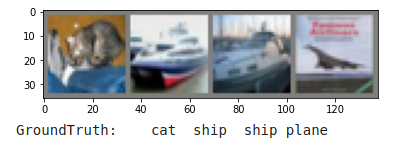
dataiter = iter(testloader)
images, labels = dataiter.next()# print images
imshow(torchvision.utils.make_grid(images))print('GroundTruth: ', ' '.join('%5s' % classes[labels[j]] for j in range(4)))

Code is available on Google Colab. That’s it I hope you enjoy and learn. This is just a simple network, I hope you add more things to this, thank you.

Disclaimer-Images without links in the caption are by the author; otherwise, a link is provided.

Join thousands of data leaders on the AI newsletter. Join over 80,000 subscribers and keep up to date with the latest developments in AI. From research to projects and ideas. If you are building an AI startup, an AI-related product, or a service, we invite you to consider becoming a sponsor.

Published via Towards AI